Compute the integrated root mean-square error

Computes the average/cumulative deviation given two continuous functions and an optional function representing the probability density function. Only one-dimensional integration is supported.

IRMSE(
  estimate,
  parameter,
  fn,
  density = function(theta, ...) 1,
  lower = -Inf,
  upper = Inf,
  ...
)

Arguments

estimate: a vector of parameter estimates
parameter: a vector of population parameters
fn: a continuous function where the first argument is to be integrated and the second argument is a vector of parameters or parameter estimates. This function represents a implied continuous function which uses the sample estimates or population parameters
density: (optional) a density function used to marginalize (i.e., average), where the first argument is to be integrated, and must be of the form density(theta, ...) or density(theta, param1, param2), where param1 is a placeholder name for the hyper-parameters associated with the probability density function. If omitted then the cumulative different between the respective functions will be computed instead
lower: lower bound to begin numerical integration from
upper: upper bound to finish numerical integration to
...: additional parameters to pass to fnest, fnparam, density, and integrate,

Value

returns a single numeric term indicating the average/cumulative deviation given the supplied continuous functions

Details

The integrated root mean-square error (IRMSE) is of the form $$IRMSE(\theta) = \sqrt{\int [f(\theta, \hat{\psi}) - f(\theta, \psi)]^2 g(\theta, ...)}$$ where $g(\theta, ...)$ is the density function used to marginalize the continuous sample ($f(\theta, \hat{\psi})$) and population ($f(\theta, \psi)$) functions.

References

Chalmers, R. P., & Adkins, M. C. (2020). Writing Effective and Reliable Monte Carlo Simulations with the SimDesign Package. The Quantitative Methods for Psychology, 16(4), 248-280. doi:10.20982/tqmp.16.4.p248

Sigal, M. J., & Chalmers, R. P. (2016). Play it again: Teaching statistics with Monte Carlo simulation. Journal of Statistics Education, 24(3), 136-156. doi:10.1080/10691898.2016.1246953

Author

Phil Chalmers rphilip.chalmers@gmail.com

Examples


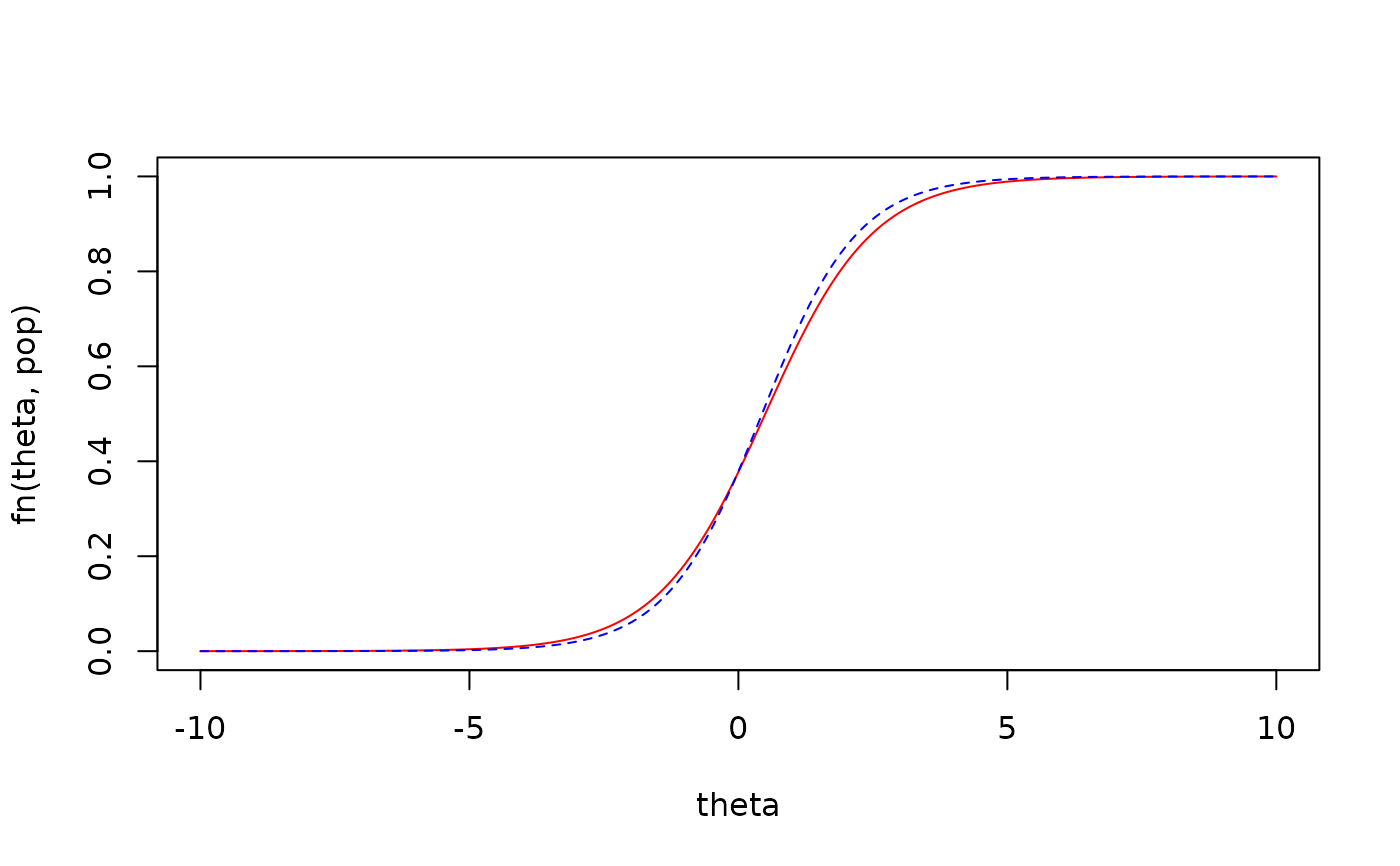
# logistic regression function with one slope and intercept
fn <- function(theta, param) 1 / (1 + exp(-(param[1] + param[2] * theta)))

# sample and population sets
est <- c(-0.4951, 1.1253)
pop <- c(-0.5, 1)

theta <- seq(-10,10,length.out=1000)
plot(theta, fn(theta, pop), type = 'l', col='red', ylim = c(0,1))
lines(theta, fn(theta, est), col='blue', lty=2)


# cumulative result (i.e., standard integral)
IRMSE(est, pop, fn)
#> [1] 0.05879362

# integrated RMSE result by marginalizing over a N(0,1) distribution
den <- function(theta, mean, sd) dnorm(theta, mean=mean, sd=sd)

IRMSE(est, pop, fn, den, mean=0, sd=1)
#> [1] 0.01933435

# this specification is equivalent to the above
den2 <- function(theta, ...) dnorm(theta, ...)

IRMSE(est, pop, fn, den2, mean=0, sd=1)
#> [1] 0.01933435