Logical Vectors, Bayesian power analyses, and ROPEs

Logical returns

In many applications it can be advantageous to directly return logical values in the simulation experiment rather than letting Spower() perform these threshold transformations internally (e.g., using sig.level) as these can include more intricate experimental requirements. The following showcases various ways that returning logical values works in the Spower package, where the average across the collected TRUE/FALSE values reflects the target power estimate.

Note that returning a logical in the simulation experiment necessarily implies that the sig.level argument in Spower() and friends will not be used, and therefore suitable alternatives must be defined within the context of the simulation experiment code (e.g., including conf.level or sig.level in the simulation experiment function directly).

Confidence (and credible) intervals

Keeping with the basic $t$ -test experiment in the introduction vignette, suppose we’re interested in the power to reject the null hypothesis $H_0:\, \mu = \mu_0$ in a one-sample $t$ -test, where $P(D|H_0)$ is the probability of the observing the data given the null hypothesis. Normally, one could simply write an experiment that returns a $p$ -value in this context, such as the following,

p_single.t <- function(n, mean, mu=0){
    g <- rnorm(n, mean=mean)
    p <- t.test(g, mu=mu)$p.value
    p
}

However, an equivalent way to explore power in this context would be to investigate the same null hypothesis via confidence intervals given a specific $\alpha$ level to define their range, where $CI_\mu=[CI_{\alpha/2},CI_{1-\alpha/2}]$ .

If one were to take this approach, the defined simulation function should return a logical value based on the relation of the parameter estimate to the CI, where the CI is used to evaluate the plausibility of $\mu = \mu_0$ . Specifically, in the context of using CI’s to reflect $p$ -value logic, the CI is used to evaluate whether $\mu_0$ falls outside the advertised interval, returning TRUE if outside the CI and FALSE if within the interval. Alternatively, if one were in a Bayesian analysis context, a credible interval could be used instead of the confidence interval to construct the same logical output.

The following code demonstrates this logic, assuming that $\alpha = .05$ (and therefore a two-tailed, 95% CI is used), and uses the is.outside_CI() function to evaluate whether the $\mu_0$ parameter falls outside the estimated CI returned from t.test().

l_single.t <- function(n, mean, mu=0, conf.level=.95){
    g <- rnorm(n, mean=mean)
    out <- t.test(g, mu=mu, conf.level=conf.level)
    CI <- out$conf.int
    is.outside_CI(mu, CI)   # equivalent to: !(CI[1] < mu && mu < CI[2])
}

l_single.t(100, mean=.2)

## [1] TRUE

Evaluating the power analysis with Spower() works out of the box now, noting again that l_single.t() will ignore the Spower(..., sig.level) information altogether as it is no longer relevant when logical information is returned. The following compares both the $p$ -value and logical CI approaches, both of which provide identical inferential information in this case (this will not always be true; the $t$ -test simply reflects a special case).

p_single.t(n=100, mean=.3) |> Spower()

## 
## Execution time (H:M:S): 00:00:03
## Design conditions: 
## 
## # A tibble: 1 × 4
##       n  mean sig.level power
##   <dbl> <dbl>     <dbl> <lgl>
## 1   100   0.3      0.05 NA   
## 
## Estimate of power: 0.846
## 95% Confidence Interval: [0.839, 0.853]

l_single.t(n=100, mean=.3) |> Spower()

## 
## Execution time (H:M:S): 00:00:04
## Design conditions: 
## 
## # A tibble: 1 × 4
##       n  mean sig.level power
##   <dbl> <dbl>     <dbl> <lgl>
## 1   100   0.3      0.05 NA   
## 
## Estimate of power: 0.841
## 95% Confidence Interval: [0.834, 0.849]

Using previouls defined simulation code

Note that even in the CI context presented above, writing user-defined functions may not be entirely necessary. This is because the related, internally defined function p_t.test() can be used to obtain the same CI information by returning the model itself, and subsequently extracting the $conf.int element. The benefit of this, as shown below, is that users do not need to reinvent the data generation and analysis portions of the experiment if this is already available in the package.

l_single.t <- function(n, mean, mu=0, conf.level=.95){
    # return analysis output from t.test() for further extraction
    out <- p_t.test(n=n, d=mean, mu=mu, type='one.sample', 
                    conf.level=conf.level, return_analysis=TRUE)
    CI <- out$conf.int
    is.outside_CI(mu, CI)
}

l_single.t(100, mean=.2)

## [1] FALSE

Precision criterion

Using confidence or credible intervals are also useful in contexts where specific precision criteria are important to satisfy. Suppose that, in addition to detecting a particular effect of interest in a given sample, the results are only deemed “practically useful” if the resulting effect size inferences are sufficiently precise, where precision could be based on the magnitude of the SE, the width of the uncertainty interval, or other relevant precision-based criterion. In this case, one may join the logic of the $p$ -value/CI approaches to create a joint evaluation for power, where a result is deemed both “significant and useful” if the null hypothesis is significantly rejected and the CI is sufficiently narrow.

As a working example, suppose that the above one-sample $t$ -test experiment was generalized such that a meaningfully significant result would require a) the rejection of the null, $\mu_0=0$ , and b) a CI width less than 1/4 standardized mean units. What value of $N$ would be required to obtain such a significant and sufficiently accurate inference to obtain a power of 80% given, say, the “small” effect size of $d=0.2$ ?

l_precision <- function(n, mean, CI.width, mu=0, alpha=.05){
    g <- rnorm(n, mean=mean)
    out <- t.test(g, mu=mu)
    CI <- out$conf.int
    width <- CI[2] - CI[1]
    # return TRUE if significant and CI is sufficiently narrow
    out$p.value < alpha && width < CI.width   
}

l_precision(n=interval(10, 500), mean=.2, CI.width=1/4) |> 
    Spower(power=.80)

# equivalently: 
# l_precision(n=NA, mean=.2, CI.width=1/4) |> 
#    Spower(power=.80, interval=c(10, 500))

## 
## Execution time (H:M:S): 00:00:22
## Design conditions: 
## 
## # A tibble: 1 × 4
##       n  mean sig.level power
##   <dbl> <dbl>     <dbl> <dbl>
## 1    NA   0.2      0.05   0.8
## 
## Estimate of n: 272.6
## 95% Predicted Confidence Interval: [272.0, 273.2]

Compared to the required $N$ from a power analysis that just contains a significant result, this joint practical significance criteria requires a meaningfully higher sample size. Note that in the special case where CI.width=Inf then all CI widths will be accepted, which will result in the same power output that would have been obtained using p_single.t().

l_precision(n=interval(10, 500), mean=.2, CI.width=Inf) |> 
    Spower(power=.80)

## 
## Execution time (H:M:S): 00:00:20
## Design conditions: 
## 
## # A tibble: 1 × 5
##       n  mean CI.width sig.level power
##   <dbl> <dbl>    <dbl>     <dbl> <dbl>
## 1    NA   0.2      Inf      0.05   0.8
## 
## Estimate of n: 198.8
## 95% Predicted Confidence Interval: [197.2, 200.2]

Bayes Factors

If one were using a Bayesian analysis criteria rather than the $p$ -value approach, the Bayes factor ( $BF$ ) ratio could be used in the logical return context too. For example, returning whether the observed $BF>3$ in a given random sample would indicate at least “moderate” supporting evidence for the hypothesis of interest compared to some competing hypothesis (often the complementary null, $P(H_0|D)$ , though not necessarily), and the average across the independent samples would indicate the degree of power when using this Bayes factor cut-off.

The downside of focusing on BFs is that they require the computation of the marginal likelihoods, typically via bridge sampling (e.g., via the bridgesampling package), in addition to fitting the model using Markov chain Monte Carlo (MCMC) methods (e.g., brms, rstan, rstanarm). Though not a strict limitation per se, it is often more natural to focus directly on the sample from posterior distribution for power analysis applications rather than on the marginal Bayes factors; this is demonstrated in the next section. Nevertheless, such applications are possible with Spower if there is sufficient interest in doing so.

As a simple example, the following one-sample $t$ -test, initially defined above, could be redefined to focus on output from the BayesFactor package, which returns the $BF$ criteria in log units (hence, exp() is used to return the ratio to its original metric) assuming a non-informative Jeffreys prior for $\mu$ . In this case a TRUE is returned if the Bayes factor is greater than 3 and FALSE if less than or equal to 3.

Finally, to ensure that nothing important is lost in the simulation experiment code a data.frame() object is returned instead of just the logical information, while Spower() is informed to only focus on the logical information for the purpose of the power computations.

l_single.Bayes.t_BF <- function(n, mean, mu=0, bf.cut=3){
    g <- rnorm(n, mean=mean)
    res <- BayesFactor::ttestBF(g, mu=mu)   
    bf <- exp(as.numeric(res@bayesFactor[1])) # Bayes factor
    data.frame(largeBF=bf > bf.cut, bf=bf)
}

Evaluating this simulation with $N=100$ , $\mu=.5$ , and $\mu_0=.3$ gives the following power estimate.

l_single.Bayes.t_BF(n=100, mean=.5, mu=.3) |> Spower(select='largeBF') -> BFsim
BFsim

## 
## Execution time (H:M:S): 00:01:24
## Design conditions: 
## 
## # A tibble: 1 × 5
##       n  mean    mu sig.level power
##   <dbl> <dbl> <dbl>     <dbl> <lgl>
## 1   100   0.5   0.3      0.05 NA   
## 
## Estimate of power: 0.265
## 95% Confidence Interval: [0.257, 0.274]

To view the complete simulation results use SimResults() on the resulting output, which if useful could be further plotted. Note that when plotting Bayes factors it is advantageous to present the plot in natural log units.

BFresults <- SimResults(BFsim)
BFresults

## # A tibble: 10,000 × 6
##        n  mean    mu sig.level largeBF      bf
##    <dbl> <dbl> <dbl>     <dbl> <lgl>     <dbl>
##  1   100   0.5   0.3      0.05 FALSE     0.131
##  2   100   0.5   0.3      0.05 FALSE     1.04 
##  3   100   0.5   0.3      0.05 FALSE     2.73 
##  4   100   0.5   0.3      0.05 TRUE     43.4  
##  5   100   0.5   0.3      0.05 FALSE     0.168
##  6   100   0.5   0.3      0.05 FALSE     1.06 
##  7   100   0.5   0.3      0.05 TRUE      3.73 
##  8   100   0.5   0.3      0.05 TRUE    442.   
##  9   100   0.5   0.3      0.05 TRUE     11.3  
## 10   100   0.5   0.3      0.05 TRUE      4.11 
## # ℹ 9,990 more rows

# use log-scale for Bayes factors as this is a more useful metric
library(ggplot2)
ggplot(BFresults, aes(log(bf), fill=largeBF)) + 
    geom_histogram(bins=50) + geom_vline(xintercept=log(3)) + 
    ggtitle('log(BF) distribution')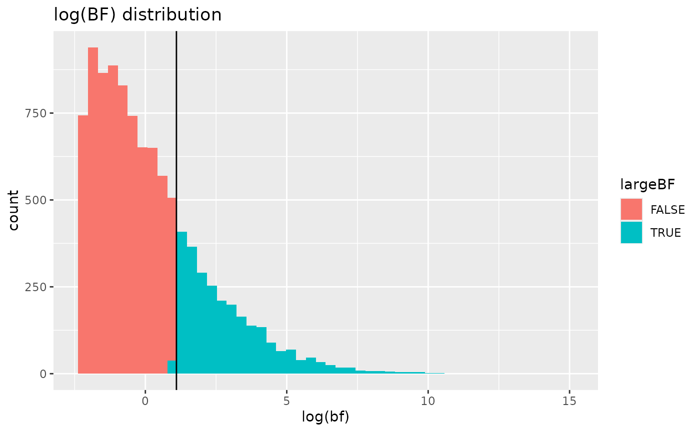

Bayesian power analysis via posterior probabiltes

The canonical way that Spower has been designed focuses primarily on $p$ -values involving the null hypothesis to be tested ( $P(D|H_0)$ ). The reason for setting the package up this way is so that the parameter $\alpha$ (sig.level) can be used as the “line-in-the-sand” threshold to flag whether a null hypothesis was rejected in each sample of data as this behaviour is common among popular power analysis software. Bayesian power analysis, on the other hand, are also supported by the package, where instead the posterior probability of the alternative hypothesis, $P(H_1|D)$ , is the focus of the simulation experiment.

Continuing with the simple one-sample $t$ -test example in the introduction vignette and above, were the power analysis context be that of a Bayesian analysis the conditional probability of the alternative, $P(H_1|D)$ , may be used instead. For this to work with Spower though, the argument sig.direction = 'above' should be supplied, where now the sig.level indicates that “significance” only occurs when an probability observation is above the define sig.level cutoff (hence, the default of .05 is no longer reasonable and should be modified).

Below is one such Bayesian approach using posterior probabilities using the BayesFactor package, which is obtained by translating the Bayes factor output into a suitable posterior probability and focusing on the alternative hypothesis (hence, the posterior probability returned corresponds to $P(\mu \ne \mu_0|D)$ ). The following also assumes that the competing hypotheses are equally likely when obtaining the posterior probability (hence, prior odds are 1:1, reflected in the argument prior_odds).

# assuming P(H1)/P(H0) are equally likely; hence, prior_odds = 1
pp_single.Bayes.t <- function(n, mean, mu, prior_odds = 1){
    g <- rnorm(n, mean=mean)
    res <- BayesFactor::ttestBF(g, mu=mu)   
    bf <- exp(as.numeric(res@bayesFactor[1])) # Bayes factor
    posterior_odds <- bf * prior_odds
    posterior <- posterior_odds / (posterior_odds + 1)   
    posterior   # P(H_1|D)
}

For the Bayesian $t$ -test definition in the next code chunk evaluation, “significance” is obtained whenever the sample posterior is greater than sig.level = .90, demonstrating strong support of $H_1$ . Note that this is a more strict criteria than the null hypothesis criteria presented in the introduction vignette, and therefore has notably lower power.

# power cut-off for a significantly supportive posterior is > 0.90
pp_single.Bayes.t(n=100, mean=.5, mu=.3) |> 
    Spower(sig.level = .90, sig.direction = 'above')

## 
## Execution time (H:M:S): 00:01:23
## Design conditions: 
## 
## # A tibble: 1 × 5
##       n  mean    mu sig.level power
##   <dbl> <dbl> <dbl>     <dbl> <lgl>
## 1   100   0.5   0.3       0.9 NA   
## 
## Estimate of power: 0.150
## 95% Confidence Interval: [0.143, 0.157]

With this approach all of the power analysis criteria described in help(Spower) are still possible, where for instance solving other experimental components (such as the sample size n) are easy to setup by providing suitable NA argument flags and search intervals in Spower().

Regions of practical equivalence (ROPEs)

This section presents two related concepts for estimating the power where some justifiable equivalence interval is of interest.

Equivalence testing

As an alternative approach to the rejection of the null hypothesis via the $p$ -value or CI approaches, there may be interest in evaluating power in the context of establishing equivalence, or in directional cases superiority or non-inferiority. The purpose of an equivalence tests is to establish that, although true differences may exist between groups, the differences are small enough to be considered “practically equivalent” in all subsequent applications.

As a running example, suppose that in an independent samples $t$ -test the two groups might be considered “equivalent” if the true mean difference in the population is somewhere above $\epsilon_L$ but below $\epsilon_U$ , where the $\epsilon$ s are used to define the equivalence interval. If, for instance, two groups are to be deemed statistically equivalent given these boundary locations then, using a two-one sided hypothesis testing approach (TOST), the two null hypotheses must be evaluated are $H_{0a}:\, (\mu_1 - \mu_2) \le -\epsilon_L$ and $H_{0b}:\,(\mu_1 - \mu_2) \ge \epsilon_U$ Rejecting both of these null hypotheses leads to the induced complementary hypothesis of interest $H_1:\, \epsilon_L < (\mu_1 - \mu_2) < \epsilon_U$ or in words, the population mean difference falls within the defined region of equivalence. Superiority testing and non-inferiority testing follow the same type of logic, however rather than defining a region of equivalence only one tail of the equivalence interval is of interest.

To put numbers to the above expression, suppose that the true mean difference between the groups was $\mu_d = \mu_2 - \mu_1 = 1$ (labeled delta), and each group had an $SD = 2.5$ (labeled sds). Furthermore, suppose any true difference that fell within the equivalence interval $[-2.5, 2.5]$ (labeled equiv) would be deemed practically equivalent a priori. The power to jointly reject the above null hypotheses, and therefore conclude the groups are practically equivalence ( $H_1$ ), is evaluated in the following output for an experiment with $N=100$ observations ( $n=50$ for each group).

l_equiv.t <- function(n, delta, equiv, sds = c(1,1), 
                      sig.level = .025){
    g1 <- rnorm(n, mean=0, sd=sds[1])
    g2 <- rnorm(n, mean=delta, sd=sds[2])
    outL <- t.test(g2, g1, mu=-equiv[1], alternative = "less")$p.value
    outU <- t.test(g2, g1, mu=equiv[2], alternative = "less")$p.value
    outL < sig.level && outU < sig.level
}

l_equiv.t(50, delta=1, equiv=c(-2.5, 2.5), 
          sds=c(2.5, 2.5)) |> Spower()

## 
## Execution time (H:M:S): 00:00:06
## Design conditions: 
## 
## # A tibble: 1 × 4
##       n delta sig.level power
##   <dbl> <dbl>     <dbl> <lgl>
## 1    50     1      0.05 NA   
## 
## Estimate of power: 0.844
## 95% Confidence Interval: [0.837, 0.851]

In this case, the power to conclude that the two groups are equivalent, expressed as a percentage, is 84%. You can verify that these computations are correct by comparing to established software for now, such as via the TOSTER package.

TOSTER::power_t_TOST(n = 50,
             delta = 1,
             sd = 2.5,
             eqb = 2.5,
             alpha = .025,
             power = NULL,
             type = "two.sample")

     Two-sample TOST power calculation 

          power = 0.8438747
           beta = 0.1561253
          alpha = 0.025
              n = 50
          delta = 1
             sd = 2.5
         bounds = -2.5, 2.5

NOTE: n is number in *each* group

Again, the same type of logic can be evaluated using CIs alone, and with the built-in p_t.test() function, where in this case TRUE is returned if the estimated 90% CI falls within the defined equivalence interval.

l_equiv.t_CI <- function(n, delta, equiv, 
                         sds = c(1,1), conf.level = .95){
    out <- p_t.test(n, delta, sds=sds, conf.level=conf.level, 
                    return_analysis=TRUE)
    is.CI_within(out$conf.int, interval=equiv)  # returns TRUE if CI is within equiv interval
}

# an equivalent power analysis for "equivalence tests" via CI evaluations
l_equiv.t_CI(50, delta=1, equiv=c(-2.5, 2.5), 
          sds=c(2.5, 2.5)) |> Spower()

## 
## Execution time (H:M:S): 00:00:05
## Design conditions: 
## 
## # A tibble: 1 × 4
##       n delta sig.level power
##   <dbl> <dbl>     <dbl> <lgl>
## 1    50     1      0.05 NA   
## 
## Estimate of power: 0.851
## 95% Confidence Interval: [0.844, 0.858]

Bayesian approach to ROPEs (HDI + ROPE)

Finally, though not exhaustively, one could approach the topic of practical equivalence using Bayesian methods using draws from the posterior distribution of interest, such as those available from BUGS or HMC samplers (e.g., stan). This approach is highly similar to the equivalence testing approach described above, but uses highest density interval + ROPE in Bayesian modeling instead. Below is one such example that constructs a simple linear regression model with a binary $X$ term that is analysed with rstanarm::stan_glm().

library(bayestestR)
library(rstanarm)

rope.lm <- function(n, beta0, beta1, range, sigma=1, ...){
    # generate data
    x <- matrix(rep(0:1, each=n))
    y <- beta0 + beta1 * x + rnorm(nrow(x), sd=sigma)
    dat <- data.frame(y, x)
    
    # run model, but tell stan_glm() to use its indoor voice
    model <- quiet(rstanarm::stan_glm(y ~ x, data = dat))
    rope <- bayestestR::rope(model, ci=1, range=range, parameters="x")
    as.numeric(rope)
}

In the above example, the proportion of the sampled posterior distribution that falls within the ROPE is returned, which works well with the sig.level argument coupled with sig.direction = 'above') in Spower() to define a suitable accept/reject cut-off. Specifically, if sig.level = .95 and sig.direction = 'above') then the ROPE will only be accepted when the percentage of the posterior distribution that falls within the defined ROPE is greater than .95. This can of course be performed manually, returning a TRUE when satisfied and FALSE otherwise, however in this case it is not necessary.

Below reports a power estimate given $N=50\times 2=100$ , where the ROPE criteria is deemed satisfied/significant if 95% of the posterior distribution for the $\beta_1=1$ falls within the defined range of $1 \pm .2\rightarrow [.8,1.2]$ . Due to the slower execution speeds of the simulations the power evaluations are computed using parallel=TRUE to utilize all available cores.

rope.lm(n=50, beta0=2, beta1=1, sigma=1/2, range=c(.8, 1.2)) |> 
    Spower(sig.level=.95, sig.direction='above', parallel=TRUE)

## 
## Execution time (H:M:S): 00:04:03
## Design conditions: 
## 
## # A tibble: 1 × 5
##       n beta0 beta1 sig.level power
##   <dbl> <dbl> <dbl>     <dbl> <lgl>
## 1    50     2     1      0.95 NA   
## 
## Estimate of power: 0.144
## 95% Confidence Interval: [0.138, 0.151]

Finally, to demonstrate why this might be useful, the following estimates the required sample size to achieve 80% power when using a 95% HDI-ROPE criteria.

rope.lm(n=interval(50, 200), beta0=2, beta1=1, sigma=1/2, range=c(.8, 1.2)) |> 
    Spower(power=.80, sig.level=.95, sig.direction='above', parallel=TRUE)

## 
## Execution time (H:M:S): 00:14:53
## Design conditions: 
## 
## # A tibble: 1 × 5
##       n beta0 beta1 sig.level power
##   <dbl> <dbl> <dbl>     <dbl> <dbl>
## 1    NA     2     1      0.95   0.8
## 
## Estimate of n: 107.7
## 95% Predicted Confidence Interval: [106.7, 108.7]

Phil Chalmers

February 13, 2026