G*Power examples evaluated with Spower

Phil Chalmers

2026-02-13

This vignette replicates several of the examples found in the G*Power manual (version 3.1). It is not meant to be exhaustive, but instead demonstrates how the presented power analyses can be computed and extended using simulation methodology by either editing the default functions found within the package, or by creating a new user-defined function for yet-to-be-defined statistical analysis contexts. Unless otherwise specified, the following analyses assume that the “significance level” (sig.level in Spower()) is set to $\alpha = .05$.

Correlation

Correlation analyses require evaluating the power associated with the hypotheses $$H_0:\, \rho-\rho_0=0$$$$H_1:\, \rho-\rho_0\ne 0$$

where $\rho$ is the population correlation and $\rho_0$ the null hypothesis constant.

Example 3.3; Difference from constant (one sample case)

The following estimates the sample size required to reject $H_0:\, \rho_0=.60$ in correlation analysis with $1-\beta=.95$ probability when $\rho=.65$.

p_r(n = interval(500, 3000), r = .65, rho = .60) |> Spower(power = .95)

## 
## Execution time (H:M:S): 00:00:22
## Design conditions: 
## 
## # A tibble: 1 × 5
##       n     r   rho sig.level power
##   <dbl> <dbl> <dbl>     <dbl> <dbl>
## 1    NA  0.65   0.6      0.05  0.95
## 
## Estimate of n: 1931.4
## 95% Predicted Confidence Interval: [1901.1, 1958.2]

# this is equivalent:
# p_r(n = NA, r = .65, rho = .60) |> 
#   Spower(power = .95, interval=c(500,3000))

G*power estimates this $n$ to be 1929 using the Fisher $z$-transformation approximation, which is what is used by the Spower definition as well.

Test against constant $\rho_0=0$

The more canonical version hypotheses involving correlation coefficients appear when $rho_0=0$, as these do not require the Fisher approximation. For instance, the power associated with $\rho = .3$ with 100 pairs of observations, tested against $\rho_0=0$, results in the following.

p_r(n = 100, r = .3) |> Spower()

## 
## Execution time (H:M:S): 00:00:11
## Design conditions: 
## 
## # A tibble: 1 × 4
##       n     r sig.level power
##   <dbl> <dbl>     <dbl> <lgl>
## 1   100   0.3      0.05 NA   
## 
## Estimate of power: 0.861
## 95% Confidence Interval: [0.854, 0.867]

Next, the sample sample size estimate required to reject $H_0:\, \rho_0=0$ in correlation analysis with $1-\beta=.95$ probability when $\rho=.3$ is expressed as

p_r(n = interval(50, 1000), r = .3) |> Spower(power = .95)

## 
## Execution time (H:M:S): 00:00:17
## Design conditions: 
## 
## # A tibble: 1 × 4
##       n     r sig.level power
##   <dbl> <dbl>     <dbl> <dbl>
## 1    NA   0.3      0.05  0.95
## 
## Estimate of n: 138.3
## 95% Predicted Confidence Interval: [136.1, 140.4]

G*power 3.1 provides the same estimate as the pwr package in this case, which for comparison is presented below.

pwr::pwr.r.test(r=.3, power=.95, n=NULL)

## 
##      approximate correlation power calculation (arctangh transformation) 
## 
##               n = 137.8
##               r = 0.3
##       sig.level = 0.05
##           power = 0.95
##     alternative = two.sided

Example 27.3; Correlation - inequality of two independent Pearson r’s

Were the correlation between two independent samples to be compared, the p_2r() simulation can be adopted. Below a sample of $N_1=206$ observations appeared in the first sample ($r=.75$), while the second sample ($r=.88$) contained only $N_2=51$ observations (hence, the ratio $N_2/N_1=51/206$). This results in the post-hoc/observed power of

p_2r(n=206, r.ab=.75, r.ab2=.88, n2_n1=51/206) |> Spower()

## 
## Execution time (H:M:S): 00:00:27
## Design conditions: 
## 
## # A tibble: 1 × 5
##       n  r.ab r.ab2 sig.level power
##   <dbl> <dbl> <dbl>     <dbl> <lgl>
## 1   206  0.75  0.88      0.05 NA   
## 
## Estimate of power: 0.727
## 95% Confidence Interval: [0.718, 0.735]

G*power 3.1 returns the power of .726 in this context.

Example 28.3.1; Correlation - inequality of two dependent Pearson r’s (no common index)

The following two examples assume the correlation matrix

# From Gpower 3.1 manual
Cp <- matrix(c(1, .5, .4, .1, 
               .5, 1, .2, -.4, 
               .4, .2, 1, .8, 
               .1, -.4, .8, 1), 4, 4)

# rearrange rows for convenience
Cp <- Cp[c(1,4,2,3), c(1,4,2,3)]
colnames(Cp) <- rownames(Cp) <- c('x1', 'y1', 'x2', 'y2')
Cp

##     x1   y1   x2  y2
## x1 1.0  0.1  0.5 0.4
## y1 0.1  1.0 -0.4 0.8
## x2 0.5 -0.4  1.0 0.2
## y2 0.4  0.8  0.2 1.0

is the population structure. For the no common index tests all of these elements are required, while for the common index form only a $3\times 3$ subset is needed.

Evaluating the null hypothesis that $$H_0: \rho_{ab} = \rho_{cd}$$ where in this case $\rho_{ab} = .5$ and $\rho_{cd} = .8$ can be explored using the p_2r() function. The following performs an a priori analyses to determine the sample size ($N$) required to achieve 80% power using Steiger’s (1980) inferential $z$ approach.

p_2r(n=interval(500, 2000), r.ab=.1, r.ac=.5, r.ad=.4, r.bc=-.4, r.bd=.8, r.cd=.2, two.tailed=FALSE) |> 
    Spower(power = .80)

## 
## Execution time (H:M:S): 00:01:36
## Design conditions: 
## 
## # A tibble: 1 × 9
##       n  r.ab  r.ac  r.ad  r.bd  r.cd two.tailed sig.level power
##   <dbl> <dbl> <dbl> <dbl> <dbl> <dbl> <lgl>          <dbl> <dbl>
## 1    NA   0.1   0.5   0.4   0.8   0.2 FALSE           0.05   0.8
## 
## Estimate of n: 886.2
## 95% Predicted Confidence Interval: [875.3, 897.3]

G*power 3.1 returns the required sample size of $N=886$.

Example 28.3.2; Correlation - inequality of two dependent Pearson r’s (common index)

The information in this example is the same as Example 28.3.1, however it is assumed that there is a common index between the correlation measures instead of a complete overlap. As such, the previous Cp object may be further subset to see what type of correlation structure is required for the common index setup.

Cp[c(4,3,1),c(4,3,1)]

##     y2  x2  x1
## y2 1.0 0.2 0.4
## x2 0.2 1.0 0.5
## x1 0.4 0.5 1.0

The null under instigation in this case is $$H_0:\rho_{ab} = \rho_{ac}$$ where $\rho_{ab} = .2$ and $\rho_{ac} = .4$. In Spower, this equates to the following inputs, which again use Steiger’s (1980) inferential $z$ approach by default.

p_2r(n=interval(50, 500), r.ab=.4, r.ac=.2, r.bc=.5, two.tailed=FALSE) |> 
    Spower(power = .80)

## 
## Execution time (H:M:S): 00:01:19
## Design conditions: 
## 
## # A tibble: 1 × 7
##       n  r.ab  r.ac  r.bc two.tailed sig.level power
##   <dbl> <dbl> <dbl> <dbl> <lgl>          <dbl> <dbl>
## 1    NA   0.4   0.2   0.5 FALSE           0.05   0.8
## 
## Estimate of n: 134.7
## 95% Predicted Confidence Interval: [133.1, 136.3]

G*power 3.1 returns the required sample size of $N=144$, which interestingly is slightly higher than the simulation version from Spower. Providing $N=144$ to the above to obtain the power estimate gives the following:

p_2r(n=144, r.ab=.4, r.ac=.2, r.bc=.5, two.tailed=FALSE) |> Spower()

## 
## Execution time (H:M:S): 00:00:22
## Design conditions: 
## 
## # A tibble: 1 × 7
##       n  r.ab  r.ac  r.bc two.tailed sig.level power
##   <dbl> <dbl> <dbl> <dbl> <lgl>          <dbl> <lgl>
## 1   144   0.4   0.2   0.5 FALSE           0.05 NA   
## 
## Estimate of power: 0.831
## 95% Confidence Interval: [0.824, 0.839]

Example 28.3.3; sensitivity analysis

It is also possible to perform a sensitivity analyses rather than the above a priori power analysis. Below fixes $N=144$, while r.ac is solved to obtain 80% power. G*power 3.1 reports that $\rho_{ac} = 0.047702$, which is confirmed using the simulation below.

# confirm solution obtained by G*power (post hoc power estimate)
p_2r(n=144, r.ab=.4, r.ac=0.047702, r.bc=-0.6, two.tailed=FALSE) |> Spower()

## 
## Execution time (H:M:S): 00:00:22
## Design conditions: 
## 
## # A tibble: 1 × 6
##       n  r.ab     r.ac two.tailed sig.level power
##   <dbl> <dbl>    <dbl> <lgl>          <dbl> <lgl>
## 1   144   0.4 0.047702 FALSE           0.05 NA   
## 
## Estimate of power: 0.815
## 95% Confidence Interval: [0.808, 0.823]

Obtaining a similar estimate using Spower() requires the following sensitivity analysis structure:

# note that interval is specified as c(upper, lower) as higher values
# of r.ac result in lower power in this context
p_2r(n=144, r.ab=.4, r.ac=interval(.4, .001), r.bc=-0.6, two.tailed=FALSE) |> 
    Spower(power = .80)

## 
## Execution time (H:M:S): 00:01:38
## Design conditions: 
## 
## # A tibble: 1 × 6
##       n  r.ab  r.ac two.tailed sig.level power
##   <dbl> <dbl> <dbl> <lgl>          <dbl> <dbl>
## 1   144   0.4    NA FALSE           0.05   0.8
## 
## Estimate of r.ac: 0.048
## 95% Predicted Confidence Interval: [0.046, 0.050]

For this example, Spower and G*power 3.1 seem to agree.

Example 16.3; Point-biserial correlation

The following estimates the sample size required to obtain a power of $1-\beta=.95$ given that $r=.25$ is the true correlation, evaluated under the null $H_0:\rho\le0$ (hence, is one-tailed) with $\alpha = .05$.

# solution per group
out <- p_t.test(r = .25, n = interval(50, 200), two.tailed=FALSE) |> 
    Spower(power = .95)
out

## 
## Execution time (H:M:S): 00:00:11
## Design conditions: 
## 
## # A tibble: 1 × 5
##       n     r two.tailed sig.level power
##   <dbl> <dbl> <lgl>          <dbl> <dbl>
## 1    NA  0.25 FALSE           0.05  0.95
## 
## Estimate of n: 81.7
## 95% Predicted Confidence Interval: [79.1, 85.4]

# total sample size required
ceiling(out$n) * 2

## [1] 164

G*power gives the result $N=164$.

Relatedly, one can specify $d$, Cohen’s standardized mean-difference effect size, instead of $r$ since $d$ will be converted to $r$ inside the p_t.test() function.

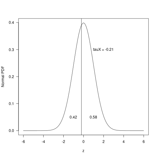
Example 31.3; tetrachoric correlation

For tetrachoric and polychoric correlations, the experiment definition in p_r.cat() can be used. This requires specifying the associated $\tau$ threshold coefficients for the population normal truncation processes, as well as the bivariate correlation itself prior to the truncation.

F <- matrix(c(203, 186, 167, 374), 2, 2)
N <- sum(F)
(marginal.x <- colSums(F)/N)

## [1] 0.4183 0.5817

(marginal.y <- rowSums(F)/N)

## [1] 0.3978 0.6022

# converted to intercepts
tauX <- qnorm(1-marginal.x)[2]
tauY <- qnorm(1-marginal.y)[2]
c(tauX, tauY)

## [1] -0.2063 -0.2589

These $\tau$ values correspond to where along the assumed normal p.d.f. the truncation took place, which for the $X$ variable can be seen in the following graphic.

Tetrachoric

Finally, assuming that the untruncated $r=0.2399846$, and a Score test were used to evaluate the null hypothesis of interest (score = TRUE), the sample size required to reject the null hypothesis that the tetrachoric correlation is less than or equal to 0 in this population (one-tailed) is expressed as

p_r.cat(n=interval(100, 500), r=0.2399846, tauX=tauX, tauY=tauY, 
        score=TRUE, two.tailed=FALSE) |> 
    Spower(power = .95, parallel=TRUE)

## 
## Design conditions: 
## 
## # A tibble: 1 × 8
##       n     r   tauX   tauY score two.tailed sig.level power
##   <dbl> <dbl> <dbl> <dbl> <lgl> <lgl>          <dbl> <dbl>
## 1    NA 0.240 -0.206 -0.259 FALSE FALSE           0.05  0.95
## 
## Estimate of n: 462.9
## 95% Prediction Interval: [458.5, 466.6]

G*power gives $n=463$, though uses the SE value at the null (Score test). p_r.cat(), on the other hand, defaults to the Wald approach where the SE is at the maximum-likelihood estimate (MLE); hence, score = FALSE by default. To switch, use score=TRUE, though note that this requires twice as many computations as a second set of data is generated and analyzed at $r=r_0$ to obtain the required $SE_0$ estimate.

Proportions

Example 4.3; One sample proportion tests

A one sample, one-tailed proportion test given data generated from a population with $\pi = .80$ and tested against the null hypothesis $H_0:\pi_0\le.65$ with $n=20$ is presented in the following. Note that G*power requires a term $g$ to be specified as the proportion difference from the null instead (hence, $g = .80-.65=.15$), though p_prop.teset() accepts the null and alternative probability values as-is.

pi <- .65
g <- .15
p <- pi + g

p_prop.test(n=20, prop=p, pi=pi, two.tailed=FALSE) |>
    Spower()

## 
## Execution time (H:M:S): 00:00:04
## Design conditions: 
## 
## # A tibble: 1 × 4
##       n two.tailed sig.level power
##   <dbl> <lgl>          <dbl> <lgl>
## 1    20 FALSE           0.05 NA   
## 
## Estimate of power: 0.416
## 95% Confidence Interval: [0.406, 0.425]

G*power gives the estimate $1-\beta=.4112$. Note that with p_prop.test(), the Fisher’s exact version of this test is also supported by passing the argument exact = TRUE.

# Fisher exact test
p_prop.test(n=20, prop=p, pi=pi, exact=TRUE, 
            two.tailed=FALSE) |> Spower()

## 
## Execution time (H:M:S): 00:00:04
## Design conditions: 
## 
## # A tibble: 1 × 5
##       n two.tailed exact sig.level power
##   <dbl> <lgl>      <lgl>     <dbl> <lgl>
## 1    20 FALSE      TRUE       0.05 NA   
## 
## Estimate of power: 0.411
## 95% Confidence Interval: [0.402, 0.421]

Example 22.1; Wilcoxon signed-rank test

The following performed a one-sample, one-tailed Wilcoxon signed rank test given $N=649$, $d=.1$, where the parent distribution is assumed to follow a Normal/Gaussian shape (default).

p_wilcox.test(n=649, d=.1, type='one.sample', two.tailed=FALSE) |> 
    Spower()

## 
## Execution time (H:M:S): 00:00:21
## Design conditions: 
## 
## # A tibble: 1 × 6
##       n     d type       two.tailed sig.level power
##   <dbl> <dbl> <chr>      <lgl>          <dbl> <lgl>
## 1   649   0.1 one.sample FALSE           0.05 NA   
## 
## Estimate of power: 0.812
## 95% Confidence Interval: [0.805, 0.820]

G*power gives the power estimate of .800.

The following partially recreates the simulation results in Figure 29 (which itself was partially extracted from Shieh, Jan, and Randles, 2007) for the Gaussian($\mu$,1) distribution with varying sample sizes and effect sizes. The target was to obtain the “approximate power of $1-\beta = .80$”, though how these sample sizes were decided upon was not specified. Spower()’s stochastic root-solving approach would likely get closer to more optimal $N$ estimates were these the target of the analyses.

# For Gaussian(d,1)
out <- p_wilcox.test(type='one.sample', two.tailed=FALSE) |> 
    SpowerBatch(n=c(649, 164, 42, 20, 12, 9),
                d=c(.1, .2, .4, .6, .8, 1.0), replications = 50000, fully.crossed=FALSE)
as.data.frame(out)

##     n   d       type two.tailed sig.level  power CI_2.5 CI_97.5
## 1 649 0.1 one.sample      FALSE      0.05 0.8012 0.7977  0.8047
## 2 164 0.2 one.sample      FALSE      0.05 0.8027 0.7992  0.8062
## 3  42 0.4 one.sample      FALSE      0.05 0.8043 0.8009  0.8078
## 4  20 0.6 one.sample      FALSE      0.05 0.8070 0.8035  0.8105
## 5  12 0.8 one.sample      FALSE      0.05 0.8018 0.7983  0.8053
## 6   9 1.0 one.sample      FALSE      0.05 0.8467 0.8435  0.8498

Laplace($\mu$, 1) version

A one-sample Wilcoxon signed rank test with Laplace distribution as the parent. Note that this requires defining the parent distribution manually, accepting arguments such as n and d.

library(extraDistr)

# generate data with scale 0-1 for d effect size to be same as mean
# VAR = 2*b^2, so scale should be 1 = 2*b^2 -> sqrt(1/2)
parent <- function(n, d, sigma=sqrt(1/2)) 
    extraDistr::rlaplace(n, d, sigma=sigma)

p_wilcox.test(n=11, d=.8, parent1=parent, type='one.sample',
              two.tailed=FALSE, correct = FALSE) |> Spower()

## 
## Execution time (H:M:S): 00:00:04
## Design conditions: 
## 
## # A tibble: 1 × 7
##       n     d type       correct two.tailed sig.level power
##   <dbl> <dbl> <chr>      <lgl>   <lgl>          <dbl> <lgl>
## 1    11   0.8 one.sample FALSE   FALSE           0.05 NA   
## 
## Estimate of power: 0.801
## 95% Confidence Interval: [0.793, 0.809]

G*power gives the estimate .830, which seems somewhat high (see below).

The following partially recreates the simulation results in Figure 29 for the Laplace($\mu$, 1) distribution with varying sample sizes and effect sizes. The target was to obtain “approximate power of $1-\beta = .80$”, though how these sample sizes were decided upon was not specified. Spower()’s stochastic root-solving approach would likely get closer to more optimal $N$ estimates were these the target of the analyses.

# For Laplace(0,1)
out <- p_wilcox.test(parent1=parent, type='one.sample',
              two.tailed=FALSE) |> 
    SpowerBatch(n=c(419, 109, 31, 16, 11, 8),
                d=c(.1, .2, .4, .6, .8, 1.0), replications=50000, fully.crossed=FALSE)
as.data.frame(out)

##     n   d       type two.tailed sig.level  power CI_2.5 CI_97.5
## 1 419 0.1 one.sample      FALSE      0.05 0.8021 0.7986  0.8056
## 2 109 0.2 one.sample      FALSE      0.05 0.7992 0.7957  0.8028
## 3  31 0.4 one.sample      FALSE      0.05 0.8031 0.7996  0.8065
## 4  16 0.6 one.sample      FALSE      0.05 0.8007 0.7972  0.8042
## 5  11 0.8 one.sample      FALSE      0.05 0.8032 0.7998  0.8067
## 6   8 1.0 one.sample      FALSE      0.05 0.7771 0.7735  0.7808

Example 5.3; Two dependent proportions test (McNemar’s test)

The following performs a proportions test between two dependent groups using McNemar’s test. The data is from O’Brien (2002, p. 161-163).

obrien2002 <- matrix(c(.54, .32, .08, .06), 2, 2,
                     dimnames = list('Treatment' = c('Yes', 'No'),
                                    'Standard' = c('Yes', 'No')))
obrien2002

##          Standard
## Treatment  Yes   No
##       Yes 0.54 0.08
##       No  0.32 0.06

p_mcnemar.test(n=50, prop=obrien2002, two.tailed=FALSE) |> Spower()

## 
## Execution time (H:M:S): 00:00:03
## Design conditions: 
## 
## # A tibble: 1 × 4
##       n two.tailed sig.level power
##   <dbl> <lgl>          <dbl> <lgl>
## 1    50 FALSE           0.05 NA   
## 
## Estimate of power: 0.836
## 95% Confidence Interval: [0.828, 0.843]

Alternatively, specifying the inputs not in terms of proportions but rather as the odds ratio ($OR=\pi_{12}/\pi_{21}=.08/.32=.25$) and proportions of discordant pairs ($\pi_D=\pi_{12} + \pi_{21}=.08 + .32=.40$) can be supplied

OR <- obrien2002[1,2] / obrien2002[2,1]
disc <- obrien2002[1,2] + obrien2002[2,1]
p_mcnemar.test(n=50, OR=OR, prop.disc=disc, two.tailed=FALSE) |> Spower()

## 
## Execution time (H:M:S): 00:00:03
## Design conditions: 
## 
## # A tibble: 1 × 4
##       n two.tailed sig.level power
##   <dbl> <lgl>          <dbl> <lgl>
## 1    50 FALSE           0.05 NA   
## 
## Estimate of power: 0.841
## 95% Confidence Interval: [0.834, 0.848]

G*Power gives .839 ($\alpha = .032$). Slightly more power can be achieved when not using the continuity correction, though in general this is not recommended in practice.

p_mcnemar.test(n=50, prop=obrien2002, two.tailed=FALSE, correct=FALSE) |> Spower()

## 
## Execution time (H:M:S): 00:00:03
## Design conditions: 
## 
## # A tibble: 1 × 5
##       n two.tailed correct sig.level power
##   <dbl> <lgl>      <lgl>       <dbl> <lgl>
## 1    50 FALSE      FALSE        0.05 NA   
## 
## Estimate of power: 0.887
## 95% Confidence Interval: [0.881, 0.893]

Multiple Linear Regression (Fixed IVs)

Example 13.1

Evaluating $R^2=.1$ generated data for a linear regression model given the null hypothesis $H_0:R^2_0=0$. When evaluated using $N=95$ observations with $k=5$ predictor variables gives the estimate.

p_lm.R2(n=95, R2=.1, k=5) |> Spower()

## 
## Execution time (H:M:S): 00:00:44
## Design conditions: 
## 
## # A tibble: 1 × 5
##       n    R2     k sig.level power
##   <dbl> <dbl> <dbl>     <dbl> <lgl>
## 1    95   0.1     5      0.05 NA   
## 
## Estimate of power: 0.664
## 95% Confidence Interval: [0.655, 0.674]

G*power gives $1-\beta = .673$.

Example 14.3

Similarly, comparing nested models for changes in $R^2$. For the following, note that k is total IVs (in this case, 9), while k.R2_0 is number of IVs for baseline model (in this case, 5). At $\alpha=.01$ and a change of $\Delta R^2=.05$ from the baseline $R^2_0=.25$ gives

p_lm.R2(n=90, R2=.3, k=9, R2_0=.25, k.R2_0=5) |> Spower(sig.level=.01)

## 
## Execution time (H:M:S): 00:00:56
## Design conditions: 
## 
## # A tibble: 1 × 7
##       n    R2     k  R2_0 k.R2_0 sig.level power
##   <dbl> <dbl> <dbl> <dbl>  <dbl>     <dbl> <lgl>
## 1    90   0.3     9  0.25      5      0.01 NA   
## 
## Estimate of power: 0.238
## 95% Confidence Interval: [0.230, 0.247]

G*power gives $1-\beta = .241$. Solving the sample size to achieve 80% power

p_lm.R2(n=interval(100, 400), R2=.3, R2_0 = .25, k=9, k.R2_0=5) |> 
        Spower(sig.level=.01, power=.8)

## 
## Execution time (H:M:S): 00:03:09
## Design conditions: 
## 
## # A tibble: 1 × 7
##       n    R2     k  R2_0 k.R2_0 sig.level power
##   <dbl> <dbl> <dbl> <dbl>  <dbl>     <dbl> <dbl>
## 1    NA   0.3     9  0.25      5      0.01   0.8
## 
## Estimate of n: 242.6
## 95% Predicted Confidence Interval: [240.5, 244.6]

G*power gives $n = 242$.

Example 14.3b

Nested model comparison for changes in $R^2$ for models with 12 IVs versus 9 IVs. Requires the specification of the $R^2_{residual}$.

p_lm.R2(n=200, R2=.16, R2_0 = .1, k=12, k.R2_0=9, R2.resid=.8) |> 
    Spower(sig.level=.01)

## 
## Execution time (H:M:S): 00:01:17
## Design conditions: 
## 
## # A tibble: 1 × 8
##       n    R2     k  R2_0 k.R2_0 R2.resid sig.level power
##   <dbl> <dbl> <dbl> <dbl>  <dbl>    <dbl>     <dbl> <lgl>
## 1   200  0.16    12   0.1      9      0.8      0.01 NA   
## 
## Estimate of power: 0.756
## 95% Confidence Interval: [0.748, 0.765]

G*power gives $1-\beta = .767$.

Multiple Linear Regression (Random IVs)

Example 7.3

Same as in Example 13.1 above, however assuming that the IVs are randomly sampled instead of fixed.

p_lm.R2(n=95, R2=.1, k=5, fixed=FALSE) |> Spower()

## 
## Execution time (H:M:S): 00:00:16
## Design conditions: 
## 
## # A tibble: 1 × 6
##       n    R2     k fixed sig.level power
##   <dbl> <dbl> <dbl> <lgl>     <dbl> <lgl>
## 1    95   0.1     5 FALSE      0.05 NA   
## 
## Estimate of power: 0.659
## 95% Confidence Interval: [0.650, 0.669]

G*power gives 0.662 using a one-tailed test criterion.

Simple linear regression

Example 12.3

Evaluate post-hoc power for simple linear regression model null hypothesis $H_0:\beta_1=0$ given $\sigma_x = 7.5$, $\sigma_y$, $\beta_1=-0.0667$, and $N=100$.

p_slr(n=100, beta=-0.0667, sd_x=7.5, sd_y = 4) |> Spower()

## 
## Execution time (H:M:S): 00:00:31
## Design conditions: 
## 
## # A tibble: 1 × 5
##       n  sd_x  sd_y sig.level power
##   <dbl> <dbl> <dbl>     <dbl> <lgl>
## 1   100   7.5     4      0.05 NA   
## 
## Estimate of power: 0.243
## 95% Confidence Interval: [0.234, 0.251]

G*power returns the power estimate $1-\beta = 0.2389$.

Fixed effects ANOVA - One way (F-test)

Example 10.3

One-way ANOVA example to solve $n$ per group (of which there are $k=10$), using Cohen’s $f=.25$, to achieve a power of $1-\beta=.95$.

p_anova.test(n=interval(20, 300), k=10, f=.25) |>  Spower(power=.95)

## 
## Execution time (H:M:S): 00:00:23
## Design conditions: 
## 
## # A tibble: 1 × 5
##       n     k     f sig.level power
##   <dbl> <dbl> <dbl>     <dbl> <dbl>
## 1    NA    10  0.25      0.05  0.95
## 
## Estimate of n: 38.7
## 95% Predicted Confidence Interval: [38.1, 39.2]

G*power gives the estimate $n=39$.

Fixing $n=200$ in total (hence, $n=200/k=20$) and performing a compromise analysis assuming $q=\frac{\beta}{\alpha}=1$,

p_anova.test(n=20, k=10, f=.25) |> Spower(beta_alpha=1, replications=30000)

## 
## Execution time (H:M:S): 00:00:44
## Design conditions: 
## 
## # A tibble: 1 × 6
##       n     k     f sig.level power beta_alpha
##   <dbl> <dbl> <dbl>     <dbl> <lgl>      <dbl>
## 1    20    10  0.25        NA NA             1
## 
## Estimate of Type I error rate (alpha/sig.level): 0.160
## 95% Confidence Interval: [0.156, 0.164]
## 
## Estimate of power (1-beta): 0.840
## 95% Confidence Interval: [0.836, 0.844]

G*Power gives $\alpha=\beta=0.159$.

$t$-test: Linear regression (two groups)

Test coefficients across distinct datasets with similar form. In this case

$$Y_1 = \beta_0 + \beta_1 X_1 + \epsilon$$$$Y_2 = \beta_0^* + \beta_1^* X_2 + \epsilon$$

where the null of interest is

$$H_0:\, \beta_1 - \beta_1^* = 0$$

To do this a multiple linear regression model is setup with three variables

$$Y = \beta_0 + \beta_1 X + \beta_2 S + \beta_3 (S\cdot X) + \epsilon$$ where $Y=[Y_1, Y_2]$, $X = [X_1, X_2]$, and $S$ is a binary indicator variable indicating whether the observations were in the second sample.

When $S = 0$ the first group’s parameterization will be recovered, while when $S=1$ the second group’s parameterization will be recovered as the potentially non-zero $\beta_2$ reflects a change in the intercept ($\beta_0^* = \beta_0 + \beta_2$) while the change in the slope for the second group will be reflected by the $\beta_3$ ($\beta_1^*=\beta_1 + \beta_3$). Hence, the null hypothesis that the two groups have the same slope can be evaluated using this augmented model by testing

$$H_0:\, \beta_3 = 0$$

Example 17.3 and 18.3

We start by defining the population generating model to replace the gen_glm() function that is the default in p_glm(). This generating function is organized such that a data.frame is returned with the columns y, X, and S, where the interaction effect reflects the magnitude of the difference between the $\beta$ coefficients across the independent samples.

gen_twogroup <- function(n, dbeta, sdx1, sdx2, sigma, n2_n1 = 1, ...){
    X1 <- rnorm(n, sd=sdx1)
    X2 <- rnorm(n*n2_n1, sd=sdx2)
    X <- c(X1, X2)
    N <- length(X)
    S <- c(rep(0, n), rep(1, N-n))
    y <- dbeta * X*S + rnorm(N, sd=sigma)
    dat <- data.frame(y, X, S)
    dat
}

To demonstrate, the post-hoc power for the described example in G*Power is the following.

p_glm(formula=y~X*S, test="X:S = 0",
      n=28, n2_n1=44/28, sdx1=9.02914, sdx2=11.86779, dbeta=0.01592,
      sigma=0.5578413, gen_fun=gen_twogroup) |> Spower()

## 
## Execution time (H:M:S): 00:00:35
## Design conditions: 
## 
## # A tibble: 1 × 8
##   test      sigma     n   sdx1   sdx2   dbeta sig.level power
##   <chr>     <dbl> <dbl>  <dbl>  <dbl>   <dbl>     <dbl> <lgl>
## 1 X:S = 0 0.55784    28 9.0291 11.868 0.01592      0.05 NA   
## 
## Estimate of power: 0.199
## 95% Confidence Interval: [0.191, 0.207]

For the a priori power analysis to achieve a power of .80

p_glm(formula=y~X*S, test="X:S = 0",
      n=interval(100, 1000), n2_n1=44/28, sdx1=9.02914, sdx2=11.86779, dbeta=0.01592,
      sigma=0.5578413, gen_fun=gen_twogroup) |> 
    Spower(power=.8)

## 
## Execution time (H:M:S): 00:02:01
## Design conditions: 
## 
## # A tibble: 1 × 8
##   test      sigma     n   sdx1   sdx2   dbeta sig.level power
##   <chr>     <dbl> <dbl>  <dbl>  <dbl>   <dbl>     <dbl> <dbl>
## 1 X:S = 0 0.55784    NA 9.0291 11.868 0.01592      0.05   0.8
## 
## Estimate of n: 164.9
## 95% Predicted Confidence Interval: [163.3, 166.8]

G*Power gives the estimate for $n$ to be 163 (and therefore 256 in the second group given the n2_n1).

Variance tests

Example 26.3; Difference from constant (one sample case)

Solve $n$ for variance ratio of $1/1.5 = 2/3$ using a one-tailed variance ratio test, assuming that the target power is $1-\beta=.80$.

p_var.test(n=interval(10, 200), vars=1, sigma2=1.5, two.tailed=FALSE) |> 
    Spower(power=.80)

## 
## Execution time (H:M:S): 00:00:34
## Design conditions: 
## 
## # A tibble: 1 × 6
##       n  vars sigma2 two.tailed sig.level power
##   <dbl> <dbl>  <dbl> <lgl>          <dbl> <dbl>
## 1    NA     1    1.5 FALSE           0.05   0.8
## 
## Estimate of n: 80.6
## 95% Predicted Confidence Interval: [79.3, 82.2]

G*power gives sample size of 81.

Example 15.3; Two-sample variance test

For a two-sample equality of variance test with equal sample sizes,

# solve n for variance ratio of 1/1.5 = 2/3, two.tailed, 80% power
p_var.test(n=interval(50, 300), vars=c(1, 1.5), two.tailed=TRUE) |> 
    Spower(power=.80)

## 
## Execution time (H:M:S): 00:00:46
## Design conditions: 
## 
## # A tibble: 1 × 4
##       n two.tailed sig.level power
##   <dbl> <lgl>          <dbl> <dbl>
## 1    NA TRUE            0.05   0.8
## 
## Estimate of n: 193.4
## 95% Predicted Confidence Interval: [191.5, 195.4]

G*Power gives estimate of 193 per group.

t-tests

Estimate sample size ($n$) per group in independent samples $t$-test, one-tailed, medium effect size ($d=0.5$), $\alpha=0.05$, 95% power ($1-\beta = 0.95$), equal sample sizes ($\frac{n_2}{n_1}=1$).

(out <- p_t.test(n = interval(10,500), d = .5, two.tailed=FALSE) |>  
               Spower(power = .95))

## 
## Execution time (H:M:S): 00:00:12
## Design conditions: 
## 
## # A tibble: 1 × 5
##       n     d two.tailed sig.level power
##   <dbl> <dbl> <lgl>          <dbl> <dbl>
## 1    NA   0.5 FALSE           0.05  0.95
## 
## Estimate of n: 86.9
## 95% Predicted Confidence Interval: [85.2, 88.5]

G*power estimate is 88 per group, Spower estimate is 86.9348 with the 95% CI [85.2011, 88.4739].

Example 19.3; Paired samples t-test

Paired-samples $t$-test, assuming the generated difference is the repeated measures Cohen’s $d_r=.421637$ (e.g., were the unadjusted $d=.4$, while $r_{xy} = .55$, then this results in the repeated $d_r=\frac{|\mu_x-\mu_y|}{\sqrt{\sigma^2_x + \sigma^2_y - 2\rho_{xy}\sigma_x\sigma_y}}$).

p_t.test(n=50 * 2, d=0.421637, type = 'paired') |> Spower(replications=50000)

## 
## Execution time (H:M:S): 00:00:22
## Design conditions: 
## 
## # A tibble: 1 × 4
##         d type   sig.level power
##     <dbl> <chr>      <dbl> <lgl>
## 1 0.42164 paired      0.05 NA   
## 
## Estimate of power: 0.840
## 95% Confidence Interval: [0.837, 0.843]

G*power gives power estimate of .832, though Cohen reported a value closer to .840. When $d=0.2828427$ this leads to

p_t.test(n=50 * 2, d=.2828427, type = 'paired') |> Spower(replications=50000)

## 
## Execution time (H:M:S): 00:00:22
## Design conditions: 
## 
## # A tibble: 1 × 4
##         d type   sig.level power
##     <dbl> <chr>      <dbl> <lgl>
## 1 0.28284 paired      0.05 NA   
## 
## Estimate of power: 0.508
## 95% Confidence Interval: [0.503, 0.512]

In this case G*Power 3.1 gives the estimate .500. To answer the question “How many subjects would we need to arrive at a power of about 0.832114 in a two-group design?” this is specified within Spower() and where n is set to NA and Spower() is passed an interval argument, or interval() is passed directly to the n element in the experiment.

p_t.test(n=interval(100,300), d=0.2828427, type = 'paired') |> 
    Spower(power=0.832114)

## 
## Execution time (H:M:S): 00:00:21
## Design conditions: 
## 
## # A tibble: 1 × 5
##       n       d type   sig.level   power
##   <dbl>   <dbl> <chr>      <dbl>   <dbl>
## 1    NA 0.28284 paired      0.05 0.83211
## 
## Estimate of n: 215.9
## 95% Predicted Confidence Interval: [213.7, 218.1]

G*power reports that around $N=110*2=220$ pairs are required, though this is estimated visually using interpolation.

Example 20.3; One-sample t-test

Evaluating the hypotheses for the mean expression $$H_0:\mu\le\mu_0$$$$H_a:\mu>\mu_0$$

using a one-sample $t$-test. The following estimates $n$ given a one-tailed $d=.625$ to achieve $1-\beta=.95$.

p_t.test(n=interval(10, 100), d=.625, two.tailed=FALSE, type='one.sample') |>  
    Spower(power=.95)

## 
## Execution time (H:M:S): 00:00:09
## Design conditions: 
## 
## # A tibble: 1 × 6
##       n     d type       two.tailed sig.level power
##   <dbl> <dbl> <chr>      <lgl>          <dbl> <dbl>
## 1    NA 0.625 one.sample FALSE           0.05  0.95
## 
## Estimate of n: 28.7
## 95% Predicted Confidence Interval: [28.0, 29.4]

G*power gives sample size of $n=30$. Similarly, though with different inputs.

p_t.test(n=interval(100,2000), d=.1, type='one.sample') |>  
    Spower(power=.9,sig.level=.01)

## 
## Execution time (H:M:S): 00:00:14
## Design conditions: 
## 
## # A tibble: 1 × 5
##       n     d type       sig.level power
##   <dbl> <dbl> <chr>          <dbl> <dbl>
## 1    NA   0.1 one.sample      0.01   0.9
## 
## Estimate of n: 1509.8
## 95% Predicted Confidence Interval: [1489.5, 1529.2]

G*power gives sample size of $n=1492$.

Wilcoxon tests

Example 22.3; One-sample test with normal distribution

Same as Example 22.1 above.

p_wilcox.test(n=649, d=.1, type='one.sample', two.tailed=FALSE) |> Spower()

## 
## Execution time (H:M:S): 00:00:21
## Design conditions: 
## 
## # A tibble: 1 × 6
##       n     d type       two.tailed sig.level power
##   <dbl> <dbl> <chr>      <lgl>          <dbl> <lgl>
## 1   649   0.1 one.sample FALSE           0.05 NA   
## 
## Estimate of power: 0.799
## 95% Confidence Interval: [0.791, 0.806]

G*power 3.1 provides a power estimate of .800, agreeing with Spower.

Similarly, assuming that the distribution for the one-sample followed a Laplace distribution, and that $N=11$ were used instead. This requires defining an alternative parent distribution, which below uses the rlaplace function from the extraDistr package.

library(extraDistr)
parent1 <- function(n, d) extraDistr::rlaplace(n, mu=d, sigma=sqrt(1/2))

# properties of sampled distribution
descript(parent1(n=100000, d=0.8))

## # A tibble: 1 × 14
##   VARS       n  miss  mean trimmed    sd   mad skewness kurtosis   min  Q_25
##   <fct>  <dbl> <dbl> <dbl>   <dbl> <dbl> <dbl>    <dbl>    <dbl> <dbl> <dbl>
## 1 df    100000    NA 0.800   0.799 0.999 0.727  0.00702     3.06 -7.94 0.309
## # ℹ 3 more variables: Q_50 <dbl>, Q_75 <dbl>, max <dbl>

p_wilcox.test(n=11, d=.8, type='one.sample', two.tailed=FALSE, parent1 = parent1) |> Spower()

## 
## Execution time (H:M:S): 00:00:04
## Design conditions: 
## 
## # A tibble: 1 × 6
##       n     d type       two.tailed sig.level power
##   <dbl> <dbl> <chr>      <lgl>          <dbl> <lgl>
## 1    11   0.8 one.sample FALSE           0.05 NA   
## 
## Estimate of power: 0.815
## 95% Confidence Interval: [0.807, 0.822]

Interestingly, G*power 3.1 reports this power to be 0.830.

Two-sample test with Laplace distributions

Two-sample Wilcoxon test comparing Laplace distributions with different central tendencies.

library(extraDistr)

parent1 <- function(n, d) extraDistr::rlaplace(n, mu=d, sigma=sqrt(1/2))
parent2 <- function(n, d) extraDistr::rlaplace(n, sigma=sqrt(1/2))

# properties of sampled distributions
descript(parent1(n=100000, d=0.375))

## # A tibble: 1 × 14
##   VARS       n  miss  mean trimmed    sd   mad skewness kurtosis   min   Q_25
##   <fct>  <dbl> <dbl> <dbl>   <dbl> <dbl> <dbl>    <dbl>    <dbl> <dbl>  <dbl>
## 1 df    100000    NA 0.381   0.382 0.997 0.725   0.0256     3.02 -6.07 -0.107
## # ℹ 3 more variables: Q_50 <dbl>, Q_75 <dbl>, max <dbl>

descript(parent1(n=100000, d=0))

## # A tibble: 1 × 14
##   VARS       n  miss    mean trimmed    sd   mad skewness kurtosis   min   Q_25
##   <fct>  <dbl> <dbl>   <dbl>   <dbl> <dbl> <dbl>    <dbl>    <dbl> <dbl>  <dbl>
## 1 df    100000    NA 0.00267 0.00272 1.000 0.726  0.00490     2.86 -8.77 -0.485
## # ℹ 3 more variables: Q_50 <dbl>, Q_75 <dbl>, max <dbl>

nr <- 134/67
p_wilcox.test(n=67, n2_n1=nr, d=0.375, parent1=parent1, parent2=parent2) |> 
    Spower()

## 
## Execution time (H:M:S): 00:00:10
## Design conditions: 
## 
## # A tibble: 1 × 4
##       n     d sig.level power
##   <dbl> <dbl>     <dbl> <lgl>
## 1    67 0.375      0.05 NA   
## 
## Estimate of power: 0.851
## 95% Confidence Interval: [0.844, 0.858]

Unlike before with the Laplace distribution, G*power 3.1 seems to agree with Spower, where a power of .847 is reported. This seems to raise questions about the consistency of the results.

Example 23.3: Paired-samples test with Laplace distributions

Finally, paired-samples approach using Wilcoxon test with $N=10$.

parent1 <- function(n, d) extraDistr::rlaplace(n, mu=d, sigma=sqrt(1/2))
parent2 <- function(n, d) extraDistr::rlaplace(n, sigma=sqrt(1/2))

descript(parent1(n=100000, d=1.13842))

## # A tibble: 1 × 14
##   VARS       n  miss  mean trimmed    sd   mad skewness kurtosis   min  Q_25
##   <fct>  <dbl> <dbl> <dbl>   <dbl> <dbl> <dbl>    <dbl>    <dbl> <dbl> <dbl>
## 1 df    100000    NA  1.14    1.14 0.996 0.727   0.0158     2.93 -7.46 0.653
## # ℹ 3 more variables: Q_50 <dbl>, Q_75 <dbl>, max <dbl>

descript(parent1(n=100000, d=0))

## # A tibble: 1 × 14
##   VARS      n  miss     mean  trimmed    sd   mad skewness kurtosis   min   Q_25
##   <fct> <dbl> <dbl>    <dbl>    <dbl> <dbl> <dbl>    <dbl>    <dbl> <dbl>  <dbl>
## 1 df      1e5    NA -0.00205 -0.00284  1.00 0.722   0.0147     3.16 -7.60 -0.490
## # ℹ 3 more variables: Q_50 <dbl>, Q_75 <dbl>, max <dbl>

p_wilcox.test(n=10*2, d=1.13842, type = 'paired',
              parent1=parent1, parent2=parent2) |> Spower()

## 
## Execution time (H:M:S): 00:00:04
## Design conditions: 
## 
## # A tibble: 1 × 4
##        d type   sig.level power
##    <dbl> <chr>      <dbl> <lgl>
## 1 1.1384 paired      0.05 NA   
## 
## Estimate of power: 0.933
## 95% Confidence Interval: [0.928, 0.938]

Again, the simulation approach and G*power 3.1 differ in their outputs, where in G*power 3.1 the reported power is 0.853.