Type M and Type S errors

Gelman, A., & Carlin, J. (2014). Beyond Power Calculations: Assessing Type S (Sign) and Type M (Magnitude) Errors. Perspectives on Psychological Science, 9(6), 641-651. https://doi.org/10.1177/1745691614551642

In the publication above, Gelman and Carlin (2014) present conditional power analysis ideas to investigate Type S and Type M errors, which add augmentations to the usual evaluation of power via the average (expected) rejection of $H_0$ or support for $H_1$ across independent samples. Specifically:

Type S errors occur when a null hypothesis is confidently rejected in light of the alternative being true, however the rejection is in the wrong direction of the underlying effect. Hence, conditional on a “statistical significance” decision, what is the probability that the correct sign was inferred?
- Ideally Type S errors should be close to 0.
- In the limiting case, where $H_0$ is true (no effect at all), then
  Type S errors will be .50 as the sign will be a coin-flip
- Type S errors are particularly prevalent in under powered research studies, where the sampling variability could result in detection of an effect that happens to be opposite what should have been detected from the population generating structure
Type M errors, on the other hand, occur when the magnitude of a detected effect is much larger than the expected effect given that “statistical significance” has occurred.
- Gelman and Carlin (2014) presented this as a ratio idea ( $M=E(\frac{|estimate|}{parameter})$ ), where large ratios indicate that the estimate had to be on average that many times higher than the expected value of the parameter (e.g., a Type M ratio of 8 indicates that of those effect sizes flagged as significant the effect estimate had to be on average 8 times larger than the true parameter).

Note that while the ratio for Type M errors gets at the idea nicely as it indicates a type of conditional “exaggeration” effect, nothing really precludes us from drawing further lines in the sand to better map this concept into a power framework. For instance, if we would only be confidence that our sample size is “large enough” if we only treat $M$ ratios less than, say, 2 or 3, then TRUE/FALSE values could be used to indicate that the observed sample has passed the desired $M$ cut-off.

Type S errors via simulation

To demonstrate how to estimate Type S errors via simulation, the following simulation experiment performs a two-sample $t$ -test with a “small” effect size (Cohen’s $d=.2$ ) with smaller sample sizes. The first implementation demonstrate the logic with a user-defined data generation and analysis, while the second approach demonstrates how the p_* functions defined within Spower can be used instead — provided that they are relevant to the power analysis under investigation.

Manual specification

In the manual implementation, where the user write both the data generation and analysis components themselves into a single function, the use of a while() loop is required to generate and analyse the experiment until a significant $p$ -value is observed. When observed, the while() loop is then terminated as the generated data matches the conditional significance criterion, at which point the subsequent analyses relevant to the compliment of Type S error (the correct sign decision) is returned as a logical so that conditional power will be reflected in the output.

l_two.t_correct.sign <- function(n, mean, mu = 0, alpha = .05, ...){
    while(TRUE){
        g1 <- rnorm(n)
        g2 <- rnorm(n, mean=mean)
        out <- t.test(g2, g1, mu=mu, ...)
        if(out$p.value < alpha) break   # if "significant" then break while() loop
    }
    mean_diff <- unname(out$estimate[1] - out$estimate[2])
    mean_diff > mu                      # return TRUE if the correct sign is observed
}

l_two.t_correct.sign(n=15, mean=.2) |> Spower()

## 
## Execution time (H:M:S): 00:00:22
## Design conditions: 
## 
## # A tibble: 1 × 4
##       n  mean sig.level power
##   <dbl> <dbl>     <dbl> <lgl>
## 1    15   0.2      0.05 NA   
## 
## Estimate of power: 0.924
## 95% Confidence Interval: [0.919, 0.929]

From the output from Spower(), the power information reflects the estimated probability that the correct sign decision was made given that “significance” was observed, while $1-power$ provides the estimate of the associated Type S error (probability of an incorrect sign given significance). As can be seen, there is about a 0.9241 probability of making the correct sign decision about the true effect, and a complimentary probability estimate of 0.0759 of making a Type S error.

With Spower, it’s of course possible to evaluate other input properties associated with these power values. For instance, suppose that we wish to know the requisite sample size such that Type S errors are made with very little frequency (hence, high conditional sign power). Further suppose we only want to make a Type S error, say, 1/100 times a significant effect is observed. The following code evaluates how to obtain such an $n$ estimate.

typeS <- .01
l_two.t_correct.sign(n=NA, mean=.2) |> 
    Spower(power=1-typeS, interval=c(10, 200))

## 
## Execution time (H:M:S): 00:00:18
## Design conditions: 
## 
## # A tibble: 1 × 4
##       n  mean sig.level power
##   <dbl> <dbl>     <dbl> <dbl>
## 1    NA   0.2      0.05  0.99
## 
## Estimate of n: 47.7
## 95% Predicted Confidence Interval: [44.1, 51.7]

Hence, one would need a sample size of approximately 48 per group in order to have a Type S error be approximately 1%.

Implementation using built-in `p_t.test()` function

Alternatively, if the simulation function and analysis already appear in the context of the package definition then Spower’s internally defined p_* functions can be used in place of the complete manual implementation. This is beneficial as the data generation and analysis components then do not need to be written by the front-end user, potentially avoiding implementation issues using previously defined simulation experiment code.

As a reminder, the default p_* functions in the package always return a $p$ -value under the null hypothesis specified as this is the canonical way in which power analysis via simulation is explored (cf. posterior probability approaches). However, these simulation experiment functions also contain a logical argument return_analysis, which if set to TRUE will return the complete analysis object instead of just the extracted $p$ -value (most commonly in the element p.value, though please use functions like str() to inspect fully). For Type M/S errors multiple components are clearly required, and therefore further information should be extracted from the analysis objects directly to accommodate.

To demonstrate, the built-in function p_t.test() is used with the return_analysis = TRUE argument. The simulation experiment still follows the while() loop logic to ensure that “significance” is first flagged, however the internal function definitions now provide the data generation and analyses so that the front-end user does not have to.

l_two.t_correct.sign <- function(n, mean, mu = 0, alpha = .05, ...){
    while(TRUE){
        # return_analysis argument used to return model object
        out <- p_t.test(n=n, d=mean, mu=mu, return_analysis=TRUE, ...)
        if(out$p.value < alpha) break
    }
    mean_diff <- unname(out$estimate[1] - out$estimate[2])
    mean_diff > mu
}

l_two.t_correct.sign(100, mean=.5)

## [1] TRUE

Setting the sample size to $N=30$ (hence, n=15) leads to the following power estimates.

l_two.t_correct.sign(n=15, mean=.2) |> Spower()

## 
## Execution time (H:M:S): 00:00:30
## Design conditions: 
## 
## # A tibble: 1 × 4
##       n  mean sig.level power
##   <dbl> <dbl>     <dbl> <lgl>
## 1    15   0.2      0.05 NA   
## 
## Estimate of power: 0.925
## 95% Confidence Interval: [0.920, 0.930]

If at all possible it is recommended to use the return_analysis approach as the simulation experiments defined within the package have all been well tested. The trade-off, as it is with all higher-level functions in R, is that there will often be slightly more overhead than user-defined functions, though of course the latter approach comes at the cost of safety.

Type M errors via simulation

Continuing with the above two-sample $t$ -test structure, suppose we’re interested in minimizing Type M errors to ensure that significant results weren’t due to higher sampling variability, ultimately resulting in significance being raised only when unreasonably large effect sizes estimates are observed. For the purpose of this power demonstration, suppose “unreasonably large” is defined such that the ratio of the absolute (standardized) mean difference in a two-sample $t$ -test, which was flagged as significant, was larger than three times the value of the true (standardized) mean difference (hence, M.ratio = 3).

Note that while focusing on an M.ratio = 3 provides the sufficient means to study Type M errors using a cut-off logic to define power, it is also possible to store the observed $M$ values for further inspection too, which can be done in Spower if a list or data.frame is returned from the supplied experiment. For this to behave correctly, however, output information relevant to the power computations (probability values/logicals) must be explicitly specified using Spower(..., select) so that other values returned from the simulation are stored but not summarised.

As before, the first step is to define the experiment using the conditional $p$ -value logic nested within a while() loop, followed by the power (and extra) criteria of interest.

l_two.t_typeM <- function(n, mean, mu = 0, 
                          alpha = .05, M.ratio = 3, ...){
    while(TRUE){
        # return_analysis argument used to return model object
        out <- p_t.test(n=n, d=mean, mu=mu, return_analysis=TRUE, ...)
        if(out$p.value < alpha) break
    }
    diff <- unname(out$estimate[1] - out$estimate[2])
    M <- abs(diff)/mean
    # return data.frame, where "retain" indicates the (logical) power information
    data.frame(retain=M < M.ratio, M=M)
}

With $N=50$ per group and a “small” standardized effect size of .2 gives the following.

# only use the "retain" information to compute power, though store the rest
l_two.t_typeM(n=50, mean=.2) |> Spower(select='retain') -> typeM
typeM

## 
## Execution time (H:M:S): 00:00:20
## Design conditions: 
## 
## # A tibble: 1 × 4
##       n  mean sig.level power
##   <dbl> <dbl>     <dbl> <lgl>
## 1    50   0.2      0.05 NA   
## 
## Estimate of power: 0.861
## 95% Confidence Interval: [0.854, 0.868]

In this case, power represents the probability that, given a significant result was observed, the resulting $M$ ratio was less than the cutoff of 3 (hence, was less than three times the true effect size). The compliment, which reflects the Type M error, is then 0.139, which is indeed quite high as approximately 14% of the samples flagged as significant would have needed rather large observed effects to indicate that the sample was “unusual” in the statistical significance sense.

With respect to the distribution of the observed $M$ values themselves, these can be further extracted using SimResults(). Notice that when plotted, the rejection magnitudes are not normally distributed, which is to be expected given the nature of the conditional simulation experiment.

results <- SimResults(typeM)
results

## # A tibble: 10,000 × 5
##        n  mean sig.level retain     M
##    <dbl> <dbl>     <dbl> <lgl>  <dbl>
##  1    50   0.2      0.05 TRUE    2.47
##  2    50   0.2      0.05 TRUE    2.44
##  3    50   0.2      0.05 TRUE    2.57
##  4    50   0.2      0.05 TRUE    2.52
##  5    50   0.2      0.05 TRUE    2.16
##  6    50   0.2      0.05 FALSE   3.59
##  7    50   0.2      0.05 TRUE    1.78
##  8    50   0.2      0.05 TRUE    2.21
##  9    50   0.2      0.05 TRUE    2.79
## 10    50   0.2      0.05 FALSE   3.38
## # ℹ 9,990 more rows

subset(results, select=M) |> descript()

## # A tibble: 1 × 14
##   VARS      n  miss  mean trimmed    sd   mad skewness kurtosis   min  Q_25
##   <fct> <dbl> <dbl> <dbl>   <dbl> <dbl> <dbl>    <dbl>    <dbl> <dbl> <dbl>
## 1 M     10000    NA  2.49    2.43 0.470 0.406     1.17     1.69  1.62  2.14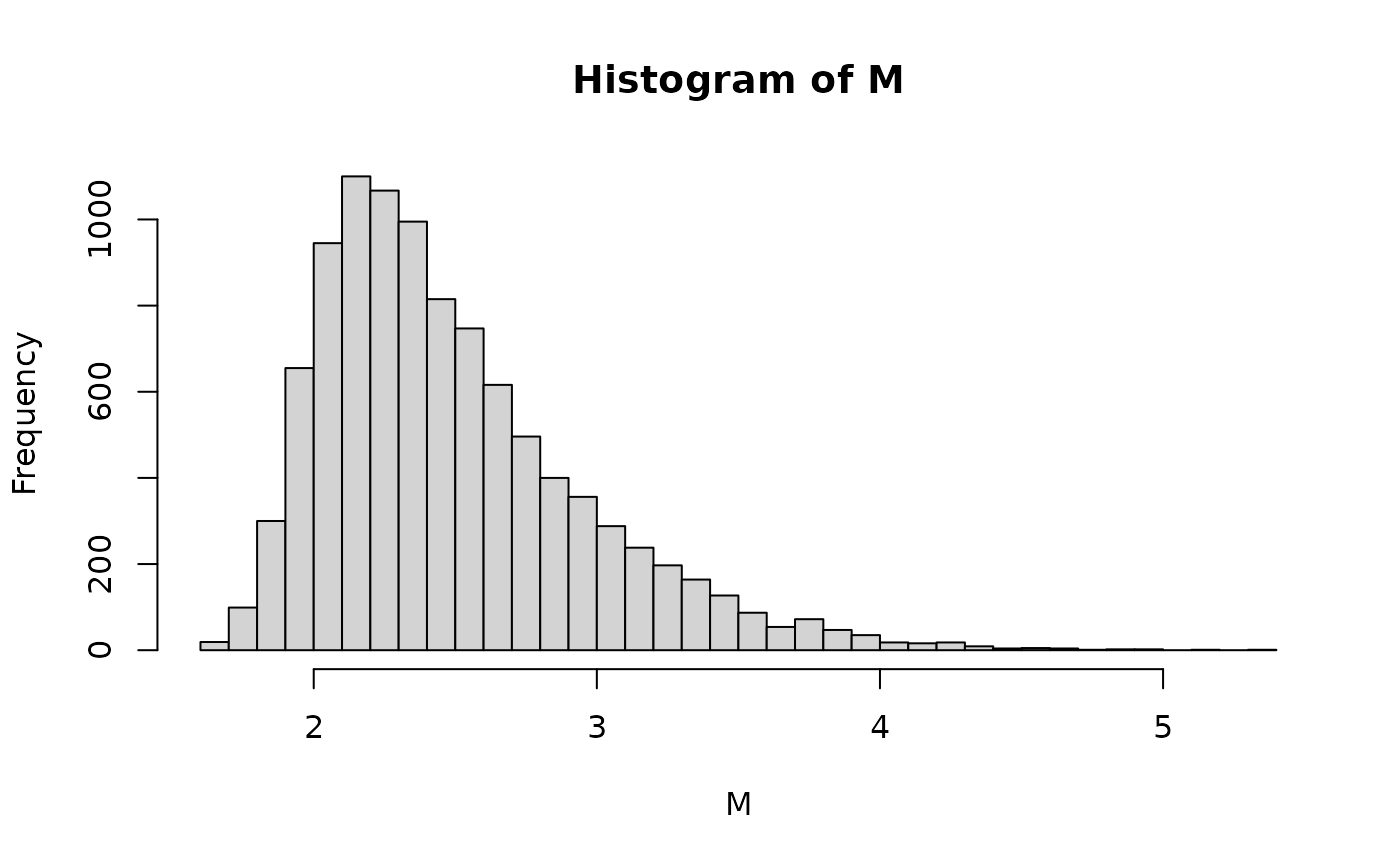
## # ℹ 3 more variables: Q_50 <dbl>, Q_75 <dbl>, max <dbl>

with(results, hist(M, 30))

Finally, increasing the sample size greatly helps with the Type M issues, as seen below by doubling the sample size below.

# double the total sample size
l_two.t_typeM(n=100, mean=.2) |> Spower(select='retain') -> typeM2
typeM2

## 
## Execution time (H:M:S): 00:00:15
## Design conditions: 
## 
## # A tibble: 1 × 4
##       n  mean sig.level power
##   <dbl> <dbl>     <dbl> <lgl>
## 1   100   0.2      0.05 NA   
## 
## Estimate of power: 0.991
## 95% Confidence Interval: [0.989, 0.993]

where the Type M error for the $M.ratio = 3$ cutoff is now

last <- getLastSpower()
1 - last$power

## [1] 0.0088

so approximately 1% of the significant results would have been due to an overly large effect size estimate. Again, the distributional properties of the observed $M$ values can be extracted and further analyzed should the need arise.

results <- SimResults(typeM2)
results

## # A tibble: 10,000 × 5
##        n  mean sig.level retain     M
##    <dbl> <dbl>     <dbl> <lgl>  <dbl>
##  1   100   0.2      0.05 TRUE    1.43
##  2   100   0.2      0.05 TRUE    1.45
##  3   100   0.2      0.05 TRUE    1.83
##  4   100   0.2      0.05 TRUE    1.72
##  5   100   0.2      0.05 TRUE    1.98
##  6   100   0.2      0.05 TRUE    1.61
##  7   100   0.2      0.05 TRUE    2.01
##  8   100   0.2      0.05 TRUE    2.52
##  9   100   0.2      0.05 TRUE    1.48
## 10   100   0.2      0.05 TRUE    1.49
## # ℹ 9,990 more rows

subset(results, select=M) |> descript()

## # A tibble: 1 × 14
##   VARS      n  miss  mean trimmed    sd   mad skewness kurtosis   min  Q_25
##   <fct> <dbl> <dbl> <dbl>   <dbl> <dbl> <dbl>    <dbl>    <dbl> <dbl> <dbl>
## 1 M     10000    NA  1.83    1.79 0.367 0.339     1.12     1.42  1.22  1.55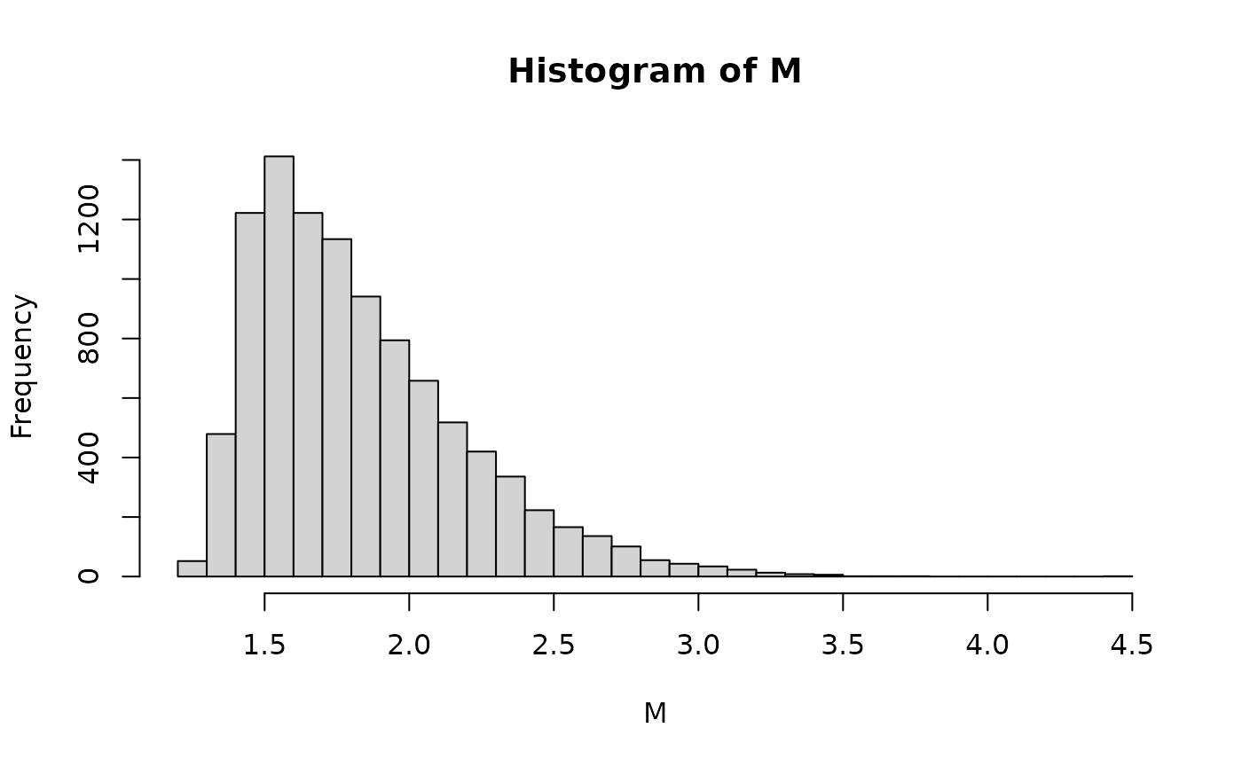
## # ℹ 3 more variables: Q_50 <dbl>, Q_75 <dbl>, max <dbl>

with(results, hist(M, 30))

Type M errors are of course intimately related to precision criteria in power analyses, and in that sense are an alternative way of looking at power planning to help from relying on “extreme” observations. Personally, the notion of thinking in terms of “ratios relative to the true population effect size” feels somewhat unnatural, though the point is obviously important as seeing significance flagged only when unreasonably large effect sizes occur is indeed troubling (e.g., replication issues).

In contrast then, I would recommend using precision-based power planning over focusing explicitly on Type M errors when power planning as this seems more natural, where obtaining greater precision in the target estimates will necessarily decrease the number of Type M error in both the “extreme” and “underwhelming” sense of the effect size estimates (the ladder of which Type M errors do not address as they do not focus on non-significant results by definition). More importantly, precis |> ion criteria are framed in the metric of the parameters relevant to the data analyst rather than on a metricless effect size ratio, which in general should be more natural to specify.

Phil Chalmers

February 13, 2026

Type S errors via simulation

Manual specification

Implementation using built-in `p_t.test()` function

Type M errors via simulation

Type M and Type S errors

Phil Chalmers

February 13, 2026

Type S errors via simulation

Manual specification

Implementation using built-in p_t.test() function

Type M errors via simulation

Implementation using built-in `p_t.test()` function