Introduction to the Spower package
Phil Chalmers
June 18, 2026
Source:vignettes/SpowerIntro.Rmd
SpowerIntro.RmdThis vignette provides a brief introduction to using the package
Spower for prospective/post-hoc, a priori, sensitivity,
criterion, and compromise power analyses. For a more detailed
description of the package structure and philosophy please refer to
associated publication (Chalmers, 2025), as well as the documentation
found within the functions; particularly, Spower(),
SpowerBatch(), and SpowerCurve().
Types of functions
There are generally two ways to go about using Spower.
The first is by utilizing one of a handful of build-in
simulation experiments with an associated data-generation and
analysis, or more flexibility (but less user friendly) by constructing a
user-defined simulation experiment by way of writing
simulation code that is encapsulated inside a single function. In either
case, the goal is to design R code to perform a given simulation
experiment with a set of meaningful (often scalar) functional arguments,
where the output from this function returns either:
- A suitable -value under the null hypothesis statistical testing (NHST) paradigm, ,
- The posterior probability of a (typically alternative) hypothesis, , or
- A logical value indicating support for the hypothesis of interest
For the first two cases, the
value returned is compared to a suitable cut-off defined by the package
(e.g., is
less than
for the first option, while the second might be
greater than
),
and therefore converted to a TRUE/FALSE value internally,
while the ladder does not require such a transformation. In all cases,
the average of the resulting TRUE/FALSE values
reflects something to do with statistical power (e.g., TRUE
if rejecting the null; TRUE if supporting the alternative;
some more complicated combination involving precision, multiple
hypotheses, regions of practical equivalence/significance, etc), thereby
forming the basis for all subsequent power analysis procedures.
The internal functions available in Spower primarily
focuses on the first approach criteria involving NHST
-values,
as this is historically the most common in similar software (e.g.,
GPower 3), however nothing precludes Spower from
more complex and interesting power analyses. See the vignette
“Logical Vectors, Bayesian power analyses and ROPEs” for more
advanced examples involving confidence intervals (CIs), parameter
precision criterion, regions of practical equivalences (ROPEs),
equivalence tests, Bayes Factors, and power analyses involving posterior
probabilities. See also the vignette “Type S and Type M errors”
for conditional power evaluation information to estimate sign (S) and
magnitude (M) power information and their respective Type S and Type M
errors (Gelman and Carlin, 2014).
Built-in simulation experiments
Spower ships with several common statistical inference
experiments, such as those involving linear regression models, mediation
analyses, ANOVAs,
-tests,
correlations, and so on. The simulation experiments are organized with
the prefix p_, followed by the name of the analysis method.
For instance,
p_lm.R2(50, k=3, R2=.3)## [1] 0.004935905performs a single simulation experiment reflecting the null hypothesis for a linear regression model with predictor variables and a sample size of .
Translating this information into a power analysis context now simply
requires passing this experiment to Spower() (the details
of which are discussed below), where by default the estimate of power
()
is returned using the default sig.level = .05.
##
## ── Spower Results ──────────────────────────────────────────────────────────────
##
## Design conditions:
##
## # A tibble: 1 × 5
##       n    R2     k sig.level power
##   <dbl> <dbl> <dbl>     <dbl> <lgl>
## 1    50   0.3     3      0.05 NA
##
## Estimate of power: 0.971
## 95% Confidence Interval: [0.968, 0.974]
## Execution time (H:M:S): 00:00:15
Each of the p_* functions return a
-value
()
as this is the general information required to evaluate statistical
power with Spower(). Alternatively, users may define their
own simulation functions if the desired experiment has not been defined
within the package.
User-defined simulation experiments
As a very simple example, suppose one were interested in the power to
reject the null hypothesis
in a one-sample
-test
scenario, where
is the probability of the data given the null hypothesis of interest.
Note that while the package already supports this type of analysis (see
help(p_t.test)) it is instructive to see how users they can
write their own version of this experiment, as this will help in
defining simulations outside what is currently included in the
package.
This simulation experiment will first obtain sample of data drawn
from a Gaussian distribution with some specific mean
(),
and evaluate the conditional probability that the data were generated
from a population with a
(the null; hence,
).
As such, the
-value
returned from this experiments reflects the probability of observing the
data given the null hypothesis
,
or more specifically
,
for a single generated dataset.
# a single experiment
p_single.t(n=100, mean=.2)
## [1] 0.06328707From here, a suitable cut-off is required to evaluate whether the
experiment was ‘significant’, which is the purpose of the parameter
.
Specifically, if the observed data
()
were plausibly drawn from a population with
(hence,
)
then a FALSE significance would be returned; otherwise, if
the data were unlikely to have been observed given the
()
then a TRUE would be returned, thereby indicating
statistical significance.
For convenience, and for the purpose of other types of specialized
power analyses (e.g., compromise analyses), the
parameter has been controlled via the argument
Spower(..., sig.level = .05), which creates the
TRUE/FALSE evaluations internally. This saves a step in the
writing, but if users wished to defined sig.level within
the simulation experiment itself that is an acceptable approach too.
Types of power analyses to evaluate
For power analyses there are typically four parameters that can be manipulated/solved in a given experiment: the level (Type I error, often reflexively set to ), power (the complement of the Type II error, ), an effect size of interest, and the sample size. Given three of these values, the fourth can always be solved.
Note that the above description reflects a general rule-of-thumb, as
there may be multiple effect sizes of interest, multiple sample size
definitions (e.g., in the form of cluster sizes in multi-level models),
and so on. Regardless, in Spower() switching between these
types of power analysis criteria is performed simply by explicitly
specifying which parameter is missing (NA), as demonstrated
below, and therefore specific naming conventions for the type of
analysis being performed is not particularly important, though the
following presentation may be instructive nonetheless.
Prospective/post-hoc power analysis
The canonical setup for Spower() will evaluate
prospective or post-hoc power, thereby obtaining the estimate
.
By default, Spower() uses
independent simulation replications to estimate the power
when this is the target criterion.
Given the above simulation definition, the following provides an estimate of power given the null hypothesis given that the data were generated from a distribution with with .
p_single.t(n=100, mean=.5, mu=.3) |> Spower() -> prospective
prospective
##
## ── Spower Results ──────────────────────────────────────────────────────────────
##
## Design conditions:
##
## # A tibble: 1 × 5
## n mean mu sig.level power
## <dbl> <dbl> <dbl> <dbl> <lgl>
## 1 100 0.5 0.3 0.05 NA
##
## Estimate of power: 0.515
## 95% Confidence Interval: [0.505, 0.525]
## Execution time (H:M:S): 00:00:01Compromise power analysis
Compromise power analysis involves manipulating the level until some sufficient balance between the Type I and Type II error rates are met, expressed in terms of the ratio .
In Spower, there are two ways to approach this
criterion. The first, which focuses on the beta_alpha ratio
at the outset, requires passing the target ratio to
Spower() using the same setup as the previous prospective
power analysis.
p_single.t(n=100, mean=.5, mu=.3) |>
    Spower(beta_alpha=4) -> compromise
compromise
##
## ── Spower Results ──────────────────────────────────────────────────────────────
##
## Design conditions:
##
## # A tibble: 1 × 6
## n mean mu sig.level power beta_alpha
## <dbl> <dbl> <dbl> <dbl> <lgl> <dbl>
## 1 100 0.5 0.3 NA NA 4
##
## Estimate of Type I error rate (alpha/sig.level): 0.093
## 95% Confidence Interval: [0.087, 0.098]
##
## Estimate of power (1-beta): 0.629
## 95% Confidence Interval: [0.620, 0.638]
## Execution time (H:M:S): 00:00:01This returns the estimated sig.level
()
and resulting
that satisfies the target
ratio
.
# satisfies q = 4 ratio
with(compromise, (1 - power) / sig.level)
## [1] 4The second way to perform a compromise analysis is to re-use a previous evaluation of a prospective/post-hoc power analysis, as this contains all the necessary information for obtaining the compromise estimates.
# using previous post-hoc/prospective power analysis
update(prospective, beta_alpha=4)
##
## ── Spower Results ──────────────────────────────────────────────────────────────
##
## Design conditions:
##
## # A tibble: 1 × 6
##       n  mean    mu sig.level power beta_alpha
##   <dbl> <dbl> <dbl>     <dbl> <lgl>      <dbl>
## 1   100   0.5   0.3        NA NA             4
##
## Estimate of Type I error rate (alpha/sig.level): 0.093
## 95% Confidence Interval: [0.088, 0.099]
##
## Estimate of power (1-beta): 0.627
## 95% Confidence Interval: [0.617, 0.636]
## Execution time (H:M:S): 00:00:01
In either case, the use of S3 generic update() function
can be beneficial as the stored result may be reused with alternative
beta_alpha values, thereby avoiding the need to estimate
new experimental data.
A priori power analysis
The goal of a priori power analysis is generally to obtain the sample size () associated with a specific power rate of interest (e.g., ), which is useful in the context of future data collection planning.
To estimate the sample size using Monte Carlo simulation experiments,
Spower() performs stochastic root solving using the
ProBABLI approach from the SimDesign package (see
SimSolve()), and therefore requires a specific search
interval to search within. The width of the interval should
reflect a plausible range where the researcher believes the solution to
lie, however this may be quite large as well as ProBABLI is less
influenced by the range of the search interval (Chalmers, 2024).
Moreover, as the algorithm is fundamentally based on bisections, the
midpoint of the specified interval should be
organized to reflect the researcher’s “best guess” of where the solution
is likely to be, though this is generally only worth considering if the
simulation experiment under evaluation is very time consuming.
Below the sample size n is solved to achieve a target
power of
,
where the solution for
was suspected to lie somewhere between the search
interval = c(20, 200), with the initial starting guess of
(quite far from the true solution, but in this case adds little to the
overall computation time).
##
## ── Spower Results ──────────────────────────────────────────────────────────────
##
## Design conditions:
##
## # A tibble: 1 × 4
##       n  mean sig.level power
##   <dbl> <dbl>     <dbl> <dbl>
## 1    NA   0.5      0.05   0.8
##
## Estimate of n: 32.8
## 95% Confidence Interval: [32.4, 33.1]
## Execution time (H:M:S): 00:00:09
Equivalently, rather than placing the interval
definition within Spower() and providing a suitable
NA placeholder to indicate which argument
interval pertains to, the function interval()
can be used directly in the experiment definition argument. Hence, the
following will be identical to the above example, though requires less
back-and-forth reading between the pipe separator.
##
## ── Spower Results ──────────────────────────────────────────────────────────────
##
## Design conditions:
##
## # A tibble: 1 × 4
##       n  mean sig.level power
##   <dbl> <dbl>     <dbl> <dbl>
## 1    NA   0.5      0.05   0.8
##
## Estimate of n: 32.8
## 95% Confidence Interval: [32.4, 33.1]
## Execution time (H:M:S): 00:00:09
Of course, the output will still be presented in terms of the
NA placeholder logic, however in this case the user does
not need to specify the NA explicitly as it is clear from
context.
Sensitivity power analysis
Similar to a priori power analysis, in that stochastic root solving is required, the target of sensitivity analysis is to locate some specific standardized or unstandardized effect size that will result in a particular power rate. This pertains to the question of how large an effect size must be in order to reliably detect the effect of interest, holding constant other information such as sample size.
Below the sample size is fixed at
,
while the interval for the standardized effect size
is searched between c(.1, 3). Note that the use of decimals
in the interval tells Spower() to use a continuous rather
than discrete search space (cf. with a priori, which uses an integer
search space for the simulation replicates).
##
## ── Spower Results ──────────────────────────────────────────────────────────────
##
## Design conditions:
##
## # A tibble: 1 × 4
##       n  mean sig.level power
##   <dbl> <dbl>     <dbl> <dbl>
## 1   100    NA      0.05   0.8
##
## Estimate of mean: 0.281
## 95% Confidence Interval: [0.280, 0.283]
## Execution time (H:M:S): 00:00:07
Equivalently, using interval() (not run).
# p_single.t(n=100, mean=interval(.1, 3)) |> Spower(power=.8)Criterion power analysis
Finally, in criterion power analysis the goal is to locate the
associated
level (sig.level) required to achieve a target power output
holding constant the other modeling information. This is done in
Spower() by setting the sig.level input to
NA while providing values for the other parameters. Note
that technically no search interval is require in this context as
necessarily lies between the interval
.
p_single.t(n=50, mean=.5) |>
    Spower(power=.8, sig.level=NA)
##
## ── Spower Results ──────────────────────────────────────────────────────────────
##
## Design conditions:
##
## # A tibble: 1 × 4
## n mean sig.level power
## <dbl> <dbl> <dbl> <dbl>
## 1 50 0.5 NA 0.8
##
## Estimate of sig.level: 0.010
## 95% Confidence Interval: [0.009, 0.010]
## Execution time (H:M:S): 00:00:06Multiple power evaluation functions
The following functions, SpowerBatch() and
SpowerCurve(), can be used to evaluate and visualize power
analysis results across a range of inputs rather than a single set of
fixed inputs. This section demonstrates their general usage, as their
specifications slightly differ from that of Spower(),
despite the fact that Spower() is the underlying estimation
engine.
SpowerBatch()
To begin, suppose that there were interest in evaluating the
p_single.t() function across multiple
inputs to obtain estimates of
.
While this could be performed using independent calls to
Spower(), the function SpowerBatch() can be
used instead, where the variable inputs can be specified in a suitable
vector format.
For instance, given the effect size , what would the power be to reject the null hypothesis across three different sample sizes, ?
p_single.t(mean=.5) |>
    SpowerBatch(n=c(30, 60, 90)) -> prospective.batch
prospective.batch
##
## ── Spower Results ──────────────────────────────────────────────────────────────
##
## Design conditions:
##
## # A tibble: 1 × 4
## n mean sig.level power
## <dbl> <dbl> <dbl> <lgl>
## 1 30 0.5 0.05 NA
##
## Estimate of power: 0.752
## 95% Confidence Interval: [0.743, 0.760]
## Execution time (H:M:S): 00:00:01
##
## ── Spower Results ──────────────────────────────────────────────────────────────
##
## Design conditions:
##
## # A tibble: 1 × 4
## n mean sig.level power
## <dbl> <dbl> <dbl> <lgl>
## 1 60 0.5 0.05 NA
##
## Estimate of power: 0.967
## 95% Confidence Interval: [0.963, 0.970]
## Execution time (H:M:S): 00:00:01
##
## ── Spower Results ──────────────────────────────────────────────────────────────
##
## Design conditions:
##
## # A tibble: 1 × 4
## n mean sig.level power
## <dbl> <dbl> <dbl> <lgl>
## 1 90 0.5 0.05 NA
##
## Estimate of power: 0.996
## 95% Confidence Interval: [0.995, 0.997]
## Execution time (H:M:S): 00:00:01This can further be coerced to a data.frame object if
there is reason to do so (e.g., for plotting purposes, though see also
SpowerCurve()).
as.data.frame(prospective.batch)## n mean sig.level power CI_2.5 CI_97.5
## 1 30 0.5 0.05 0.7516 0.7431313 0.7600687
## 2 60 0.5 0.05 0.9669 0.9633937 0.9704063
## 3 90 0.5 0.05 0.9963 0.9951100 0.9974900Similarly, if the were related to a priori analyses for sample size
planning then the inputs to SpowerBatch() would be modified
to set n to the missing quantity.
apriori.batch <- p_single.t(mean=.5, n=NA) |>
    SpowerBatch(power=c(.7, .8, .9), interval=c(20, 200))
apriori.batch
##
## ── Spower Results ──────────────────────────────────────────────────────────────
##
## Design conditions:
##
## # A tibble: 1 × 4
## n mean sig.level power
## <dbl> <dbl> <dbl> <dbl>
## 1 NA 0.5 0.05 0.7
##
## Estimate of n: 26.7
## 95% Confidence Interval: [26.5, 27.0]
## Execution time (H:M:S): 00:00:15
##
## ── Spower Results ──────────────────────────────────────────────────────────────
##
## Design conditions:
##
## # A tibble: 1 × 4
## n mean sig.level power
## <dbl> <dbl> <dbl> <dbl>
## 1 NA 0.5 0.05 0.8
##
## Estimate of n: 33.3
## 95% Confidence Interval: [32.9, 33.7]
## Execution time (H:M:S): 00:00:07
##
## ── Spower Results ──────────────────────────────────────────────────────────────
##
## Design conditions:
##
## # A tibble: 1 × 4
## n mean sig.level power
## <dbl> <dbl> <dbl> <dbl>
## 1 NA 0.5 0.05 0.9
##
## Estimate of n: 44.4
## 95% Confidence Interval: [43.8, 44.8]
## Execution time (H:M:S): 00:00:11
as.data.frame(apriori.batch)## n mean sig.level power CI_2.5 CI_97.5
## 1 26.71726 0.5 0.05 0.7 26.46683 26.96011
## 2 33.31082 0.5 0.05 0.8 32.90640 33.69844
## 3 44.36998 0.5 0.05 0.9 43.76155 44.84176SpowerCurve()
Often times researchers wish to visualize the results of power
analyses in the form of graphical representations. Spower
supports various types of visualizations through the function
SpowerCurve(), which creates power curve plots of
previously obtained results (e.g., via SpowerBatch()) or
for to-be-explored inputs. Importantly, each graphic contains estimates
of the Monte Carlo sampling uncertainty to deter over-interpretation of
any resulting point-estimates.
To demonstrate, suppose one were interested in visualizing the power
for the running single-sample
test across four different sample sizes,
.
To do this requires passing the simulation experiment and varying
information to the function SpowerCurve(), which fills in
the variable information to the supplied simulation experiment and plots
the resulting output.
p_single.t(mean=.5) |>
    SpowerCurve(n=c(30, 60, 90, 120))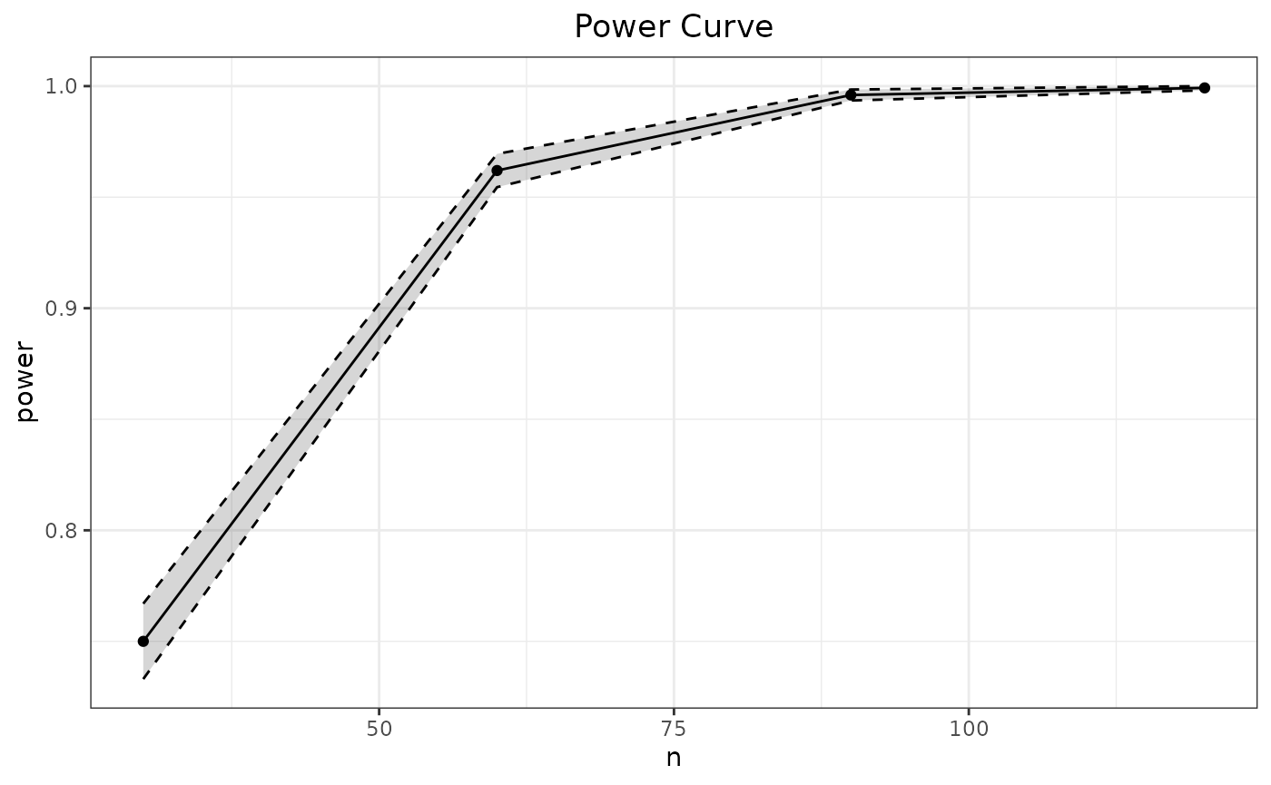
Alternatively, were the above information already evaluated using
SpowerBatch() then this batch object could be
passed directly to SpowerCurve()’s argument
batch, thereby avoiding the need to re-evaluate the
simulation experiments.
# pass previous SpowerBatch() object
SpowerCurve(batch=batch)
SpowerCurve() will accept as many arguments as exists in
the supplied simulation experiment definition, however it will only
provide aesthetic mappings for the first three variable input
specifications as anything past this becomes more difficult to display
automatically. Below is an example that varies both the n
input as well as the input mean, where the first input
appears on the
-axis
while the second is mapped to the default colour aesthetic in
ggplot2.
p_single.t() |>
    SpowerCurve(n=c(30, 60, 90, 120), mean=c(.2, .5, .8))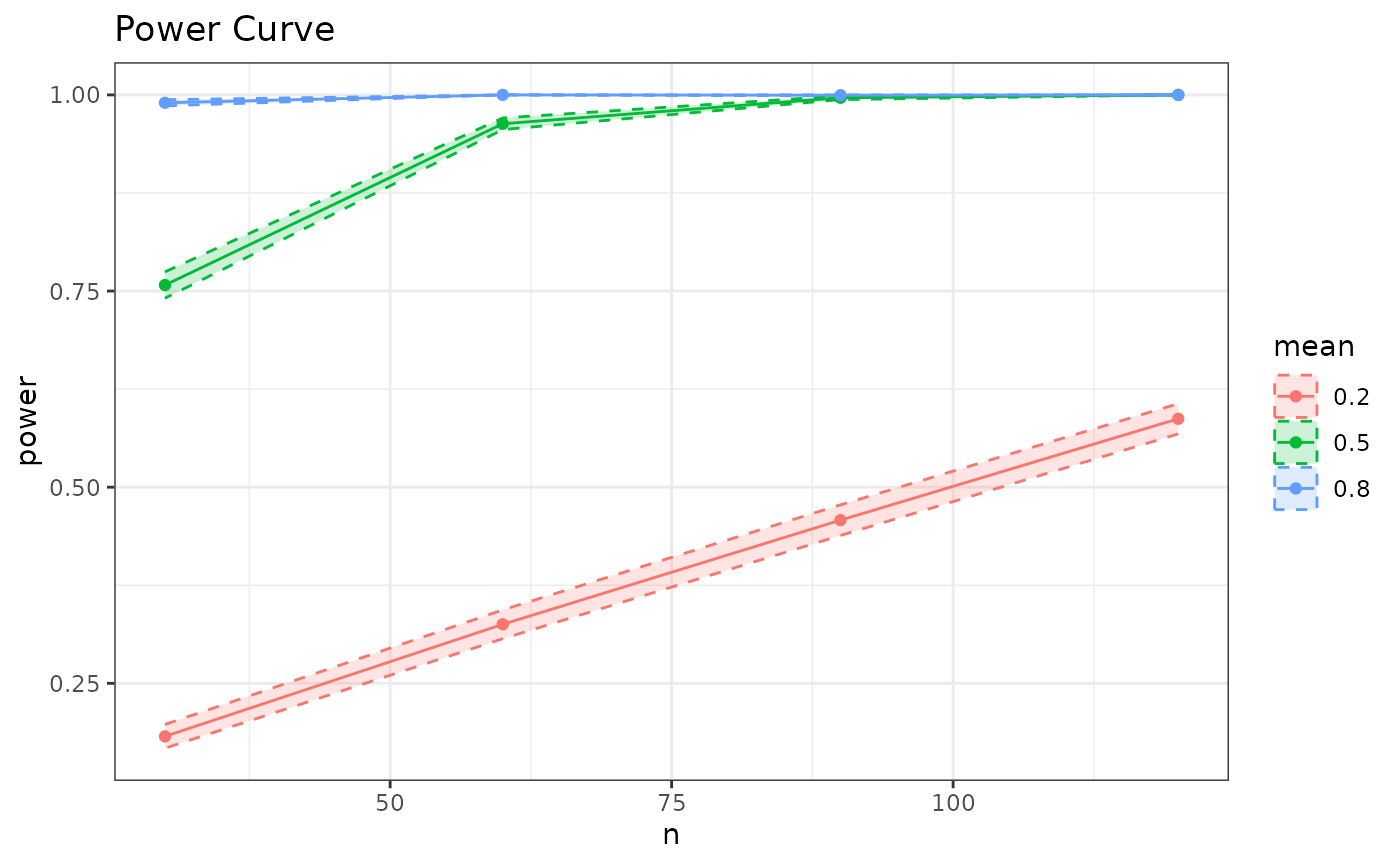
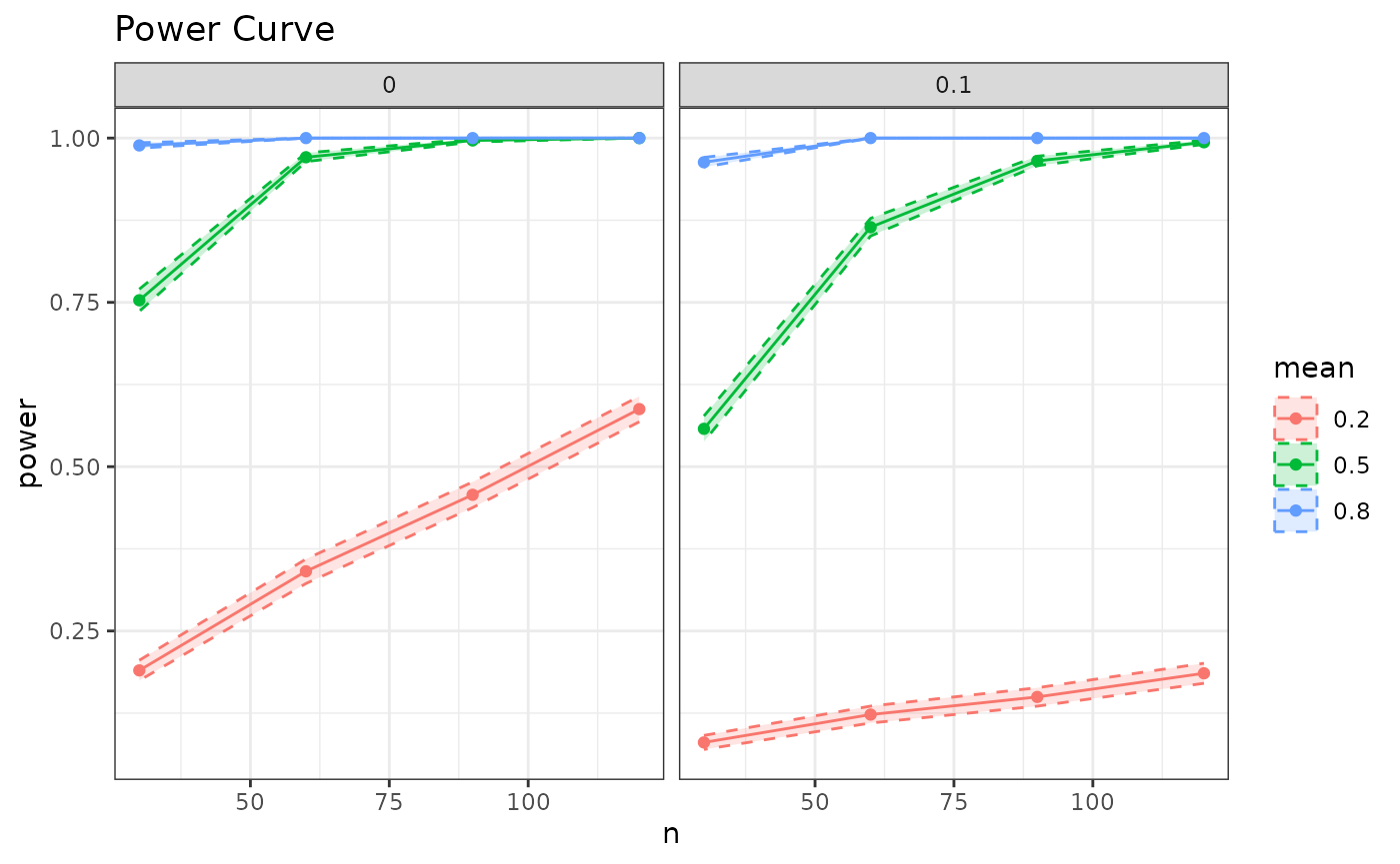
Finally, the function SpowerCurve() currently supports
up to three argument variations, where the third variable is treated as
a facet. Should other plots be require then this will fall on the user
to customize with SpowerBatch() as the types of
visualizations past three variables can become convoluted.
p_single.t() |>
    SpowerCurve(n=c(30, 60, 90, 120), mean=c(.2, .5, .8), mu=c(0, .1))