Function to generate empirical unidimensional item and test plots
Source:R/empirical_plot.R
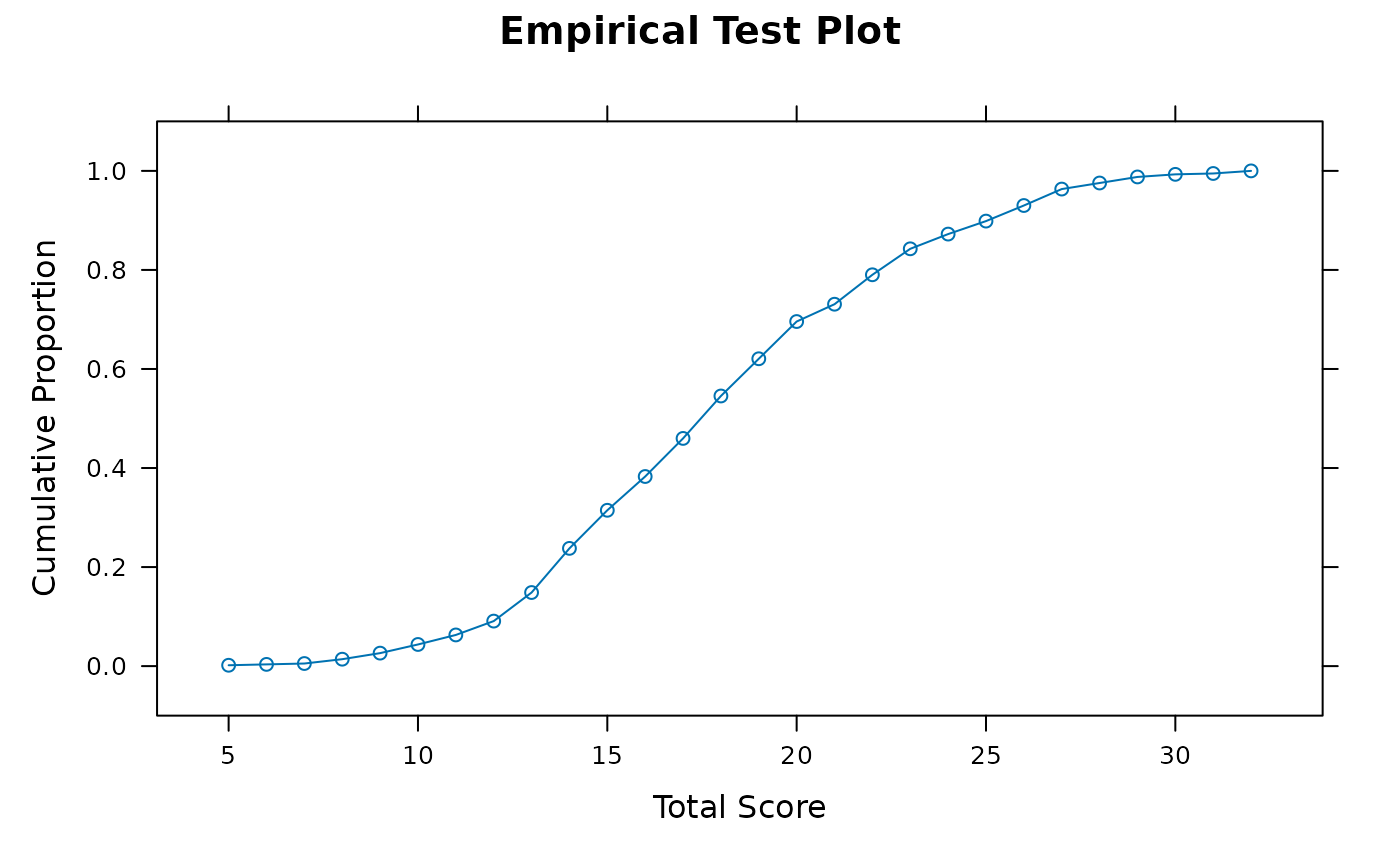
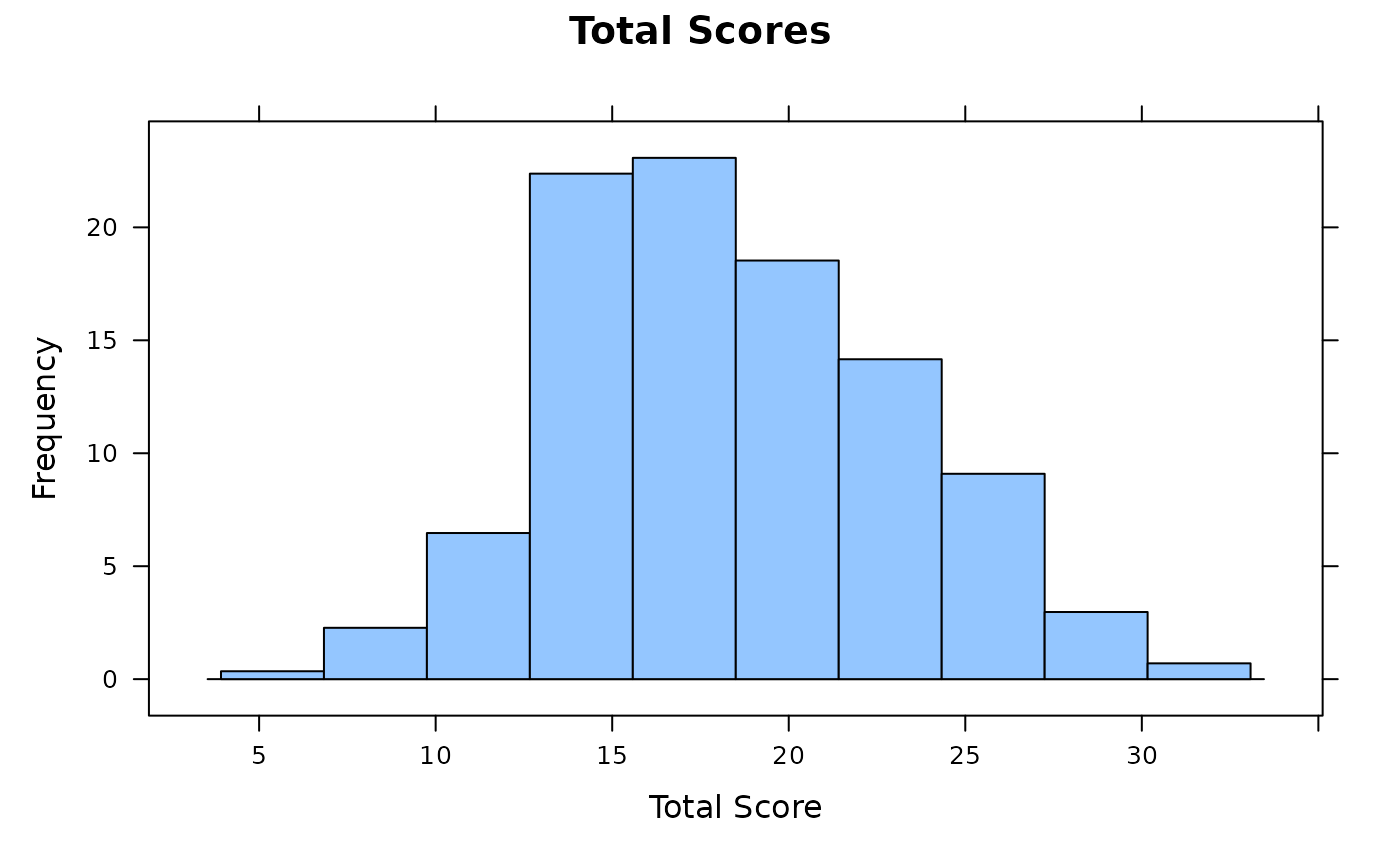
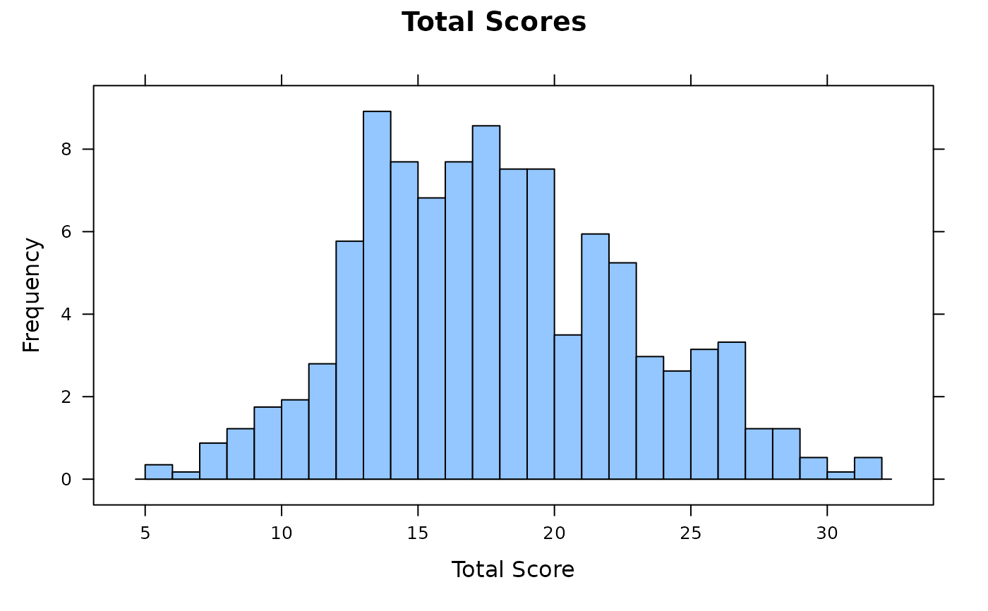
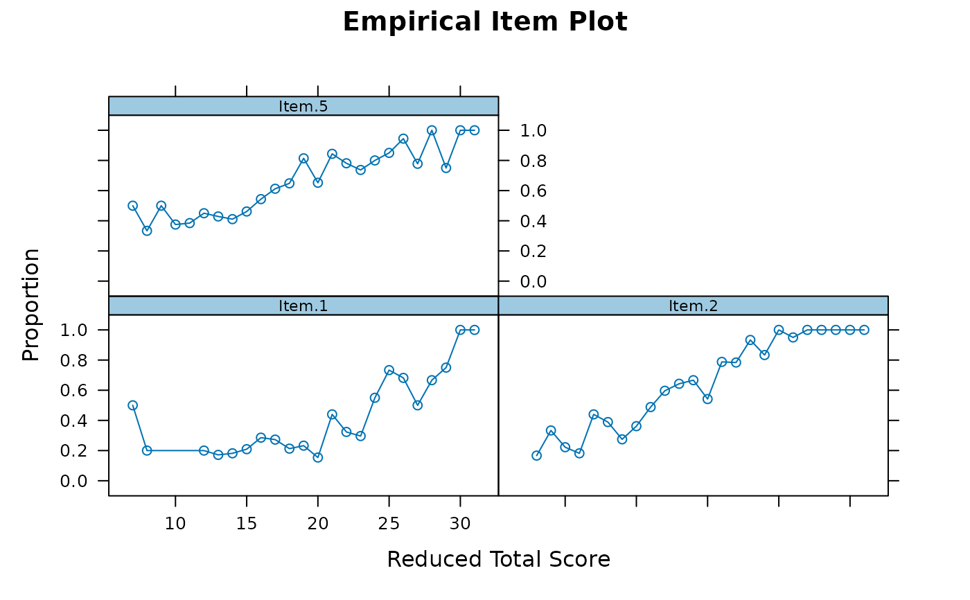
empirical_plot.RdGiven a dataset containing item responses this function will construct empirical graphics using the observed responses to each item conditioned on the total score. When individual item plots are requested then the total score will be formed without the item of interest (i.e., the total score without that item).
Usage
empirical_plot(
  data,
  which.items = NULL,
  type = "prop",
  smooth = FALSE,
  formula = resp ~ s(TS, k = 5),
  main = NULL,
  par.strip.text = list(cex = 0.7),
  par.settings = list(strip.background = list(col = "#9ECAE1"), strip.border = list(col =
    "black")),
  auto.key = list(space = "right", points = FALSE, lines = TRUE),
  ...
)
Arguments
- data
a
data.frameormatrixof item responses (seemirtfor typical input)- which.items
a numeric vector indicating which items to plot in a faceted image plot. If NULL then empirical test plots will be constructed instead
- type
character vector specifying type of plot to draw. When
which.itemis NULL can be 'prop' (default) or 'hist', otherwise can be 'prop' (default) or 'boxplot'- smooth
logical; include a GAM smoother instead of the raw proportions? Default is FALSE
- formula
formula used for the GAM smoother
- main
the main title for the plot. If NULL an internal default will be used
- par.strip.text
plotting argument passed to
lattice- par.settings
plotting argument passed to
lattice- auto.key
plotting argument passed to
lattice- ...
Details
Note that these types of plots should only be used for unidimensional tests with monotonically increasing item response functions. If monotonicity is not true for all items, however, then these plots may serve as a visual diagnostic tool so long as the majority of items are indeed monotonic.
References
Chalmers, R., P. (2012). mirt: A Multidimensional Item Response Theory Package for the R Environment. Journal of Statistical Software, 48(6), 1-29. doi:10.18637/jss.v048.i06
Examples
# \donttest{
SAT12[SAT12 == 8] <- NA
data <- key2binary(SAT12,
key = c(1,4,5,2,3,1,2,1,3,1,2,4,2,1,5,3,4,4,1,4,3,3,4,1,3,5,1,3,1,5,4,5))
# test plot
empirical_plot(data)
 empirical_plot(data, type = 'hist')
 empirical_plot(data, type = 'hist', breaks=20)
 # items 1, 2 and 5
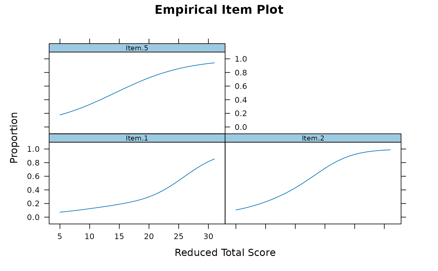
empirical_plot(data, c(1, 2, 5))
 empirical_plot(data, c(1, 2, 5), smooth = TRUE)
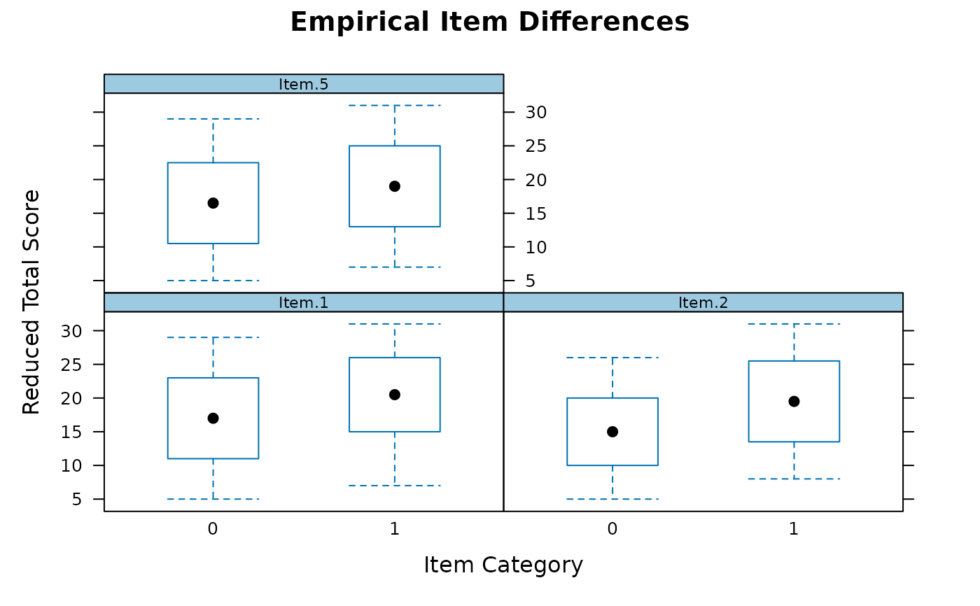
 empirical_plot(data, c(1, 2, 5), type = 'boxplot')
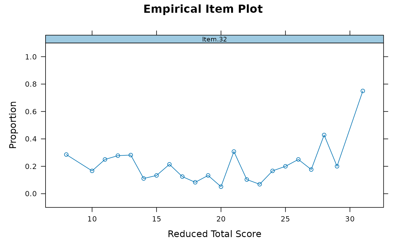
 # replace weird looking items with unscored versions for diagnostics
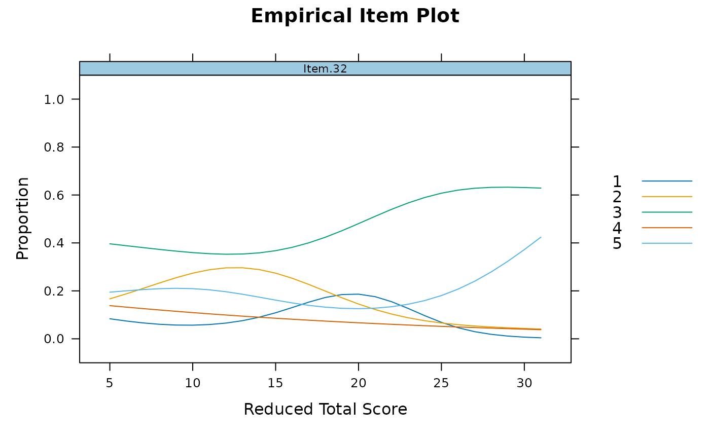
empirical_plot(data, 32)
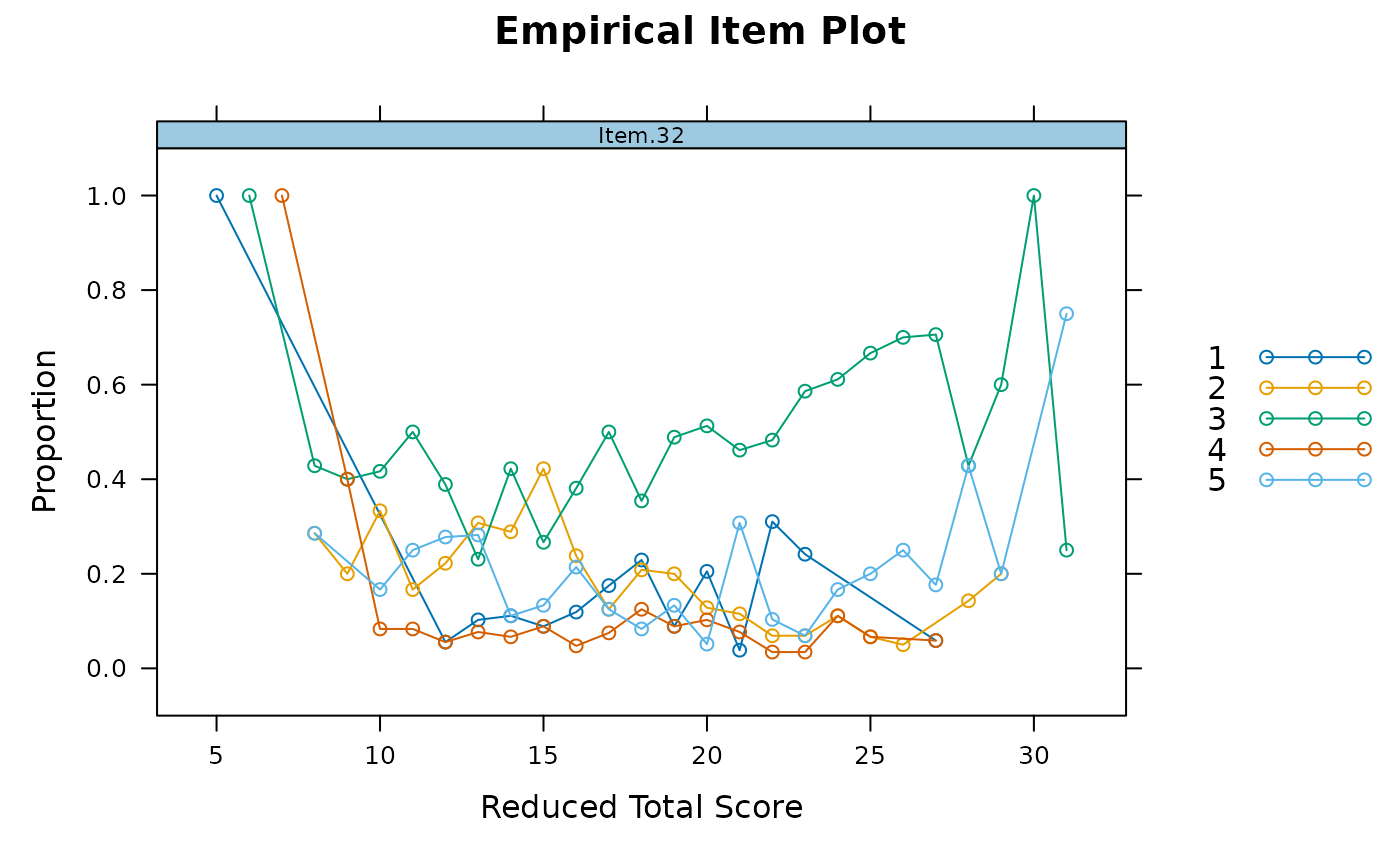
 data[,32] <- SAT12[,32]
empirical_plot(data, 32)
 empirical_plot(data, 32, smooth = TRUE)
 # }
# }