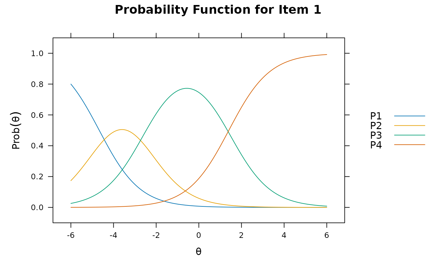
itemplot displays various item based IRT plots, with special options for plotting items
that contain several 0 slope parameters. Supports up to three dimensional models.
Usage
itemplot(
  object,
  item,
  type = "trace",
  degrees = 45,
  CE = FALSE,
  CEalpha = 0.05,
  CEdraws = 1000,
  drop.zeros = FALSE,
  theta_lim = c(-6, 6),
  shiny = FALSE,
  rot = list(xaxis = -70, yaxis = 30, zaxis = 10),
  par.strip.text = list(cex = 0.7),
  npts = 200,
  par.settings = list(strip.background = list(col = "#9ECAE1"), strip.border = list(col =
    "black")),
  auto.key = list(space = "right", points = FALSE, lines = TRUE),
  ...
)
Arguments
- object
a computed model object of class
SingleGroupClassorMultipleGroupClass. Input may also be alistfor comparing similar item types (e.g., 1PL vs 2PL)- item
a single numeric value, or the item name, indicating which item to plot
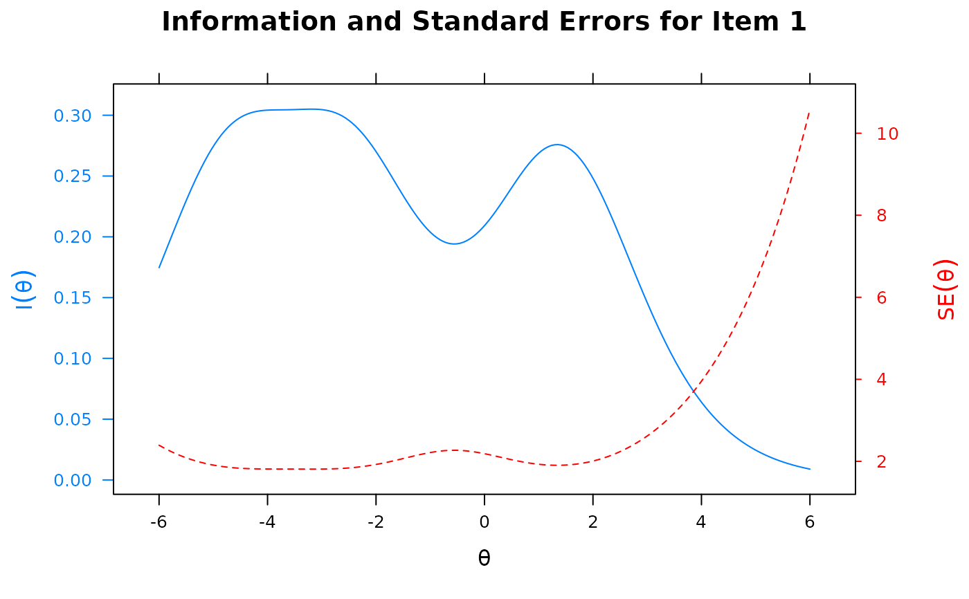
- type
plot type to use, information (
'info'), standard errors ('SE'), item trace lines ('trace'), cumulative probability plots to indicate thresholds ('threshold'), information and standard errors ('infoSE') or information and trace lines ('infotrace'), category and total information ('infocat'), relative efficiency lines ('RE'), expected score'score', or information and trace line contours ('infocontour'and'tracecontour'; not supported forMultipleGroupClassobjects)- degrees
the degrees argument to be used if there are two or three factors. See
iteminfofor more detail. A new vector will be required for three dimensional models to override the default- CE
logical; plot confidence envelope?
- CEalpha
area remaining in the tail for confidence envelope. Default gives 95% confidence region
- CEdraws
draws number of draws to use for confidence envelope
- drop.zeros
logical; drop slope values that are numerically close to zero to reduce dimensionality? Useful in objects returned from
bfactoror other confirmatory models that contain several zero slopes- theta_lim
lower and upper limits of the latent trait (theta) to be evaluated, and is used in conjunction with
npts. Default usesc(-6,6)- shiny
logical; run interactive display for item plots using the
shinyinterface. This primarily is an instructive tool for demonstrating how item response curves behave when adjusting their parameters- rot
a list of rotation coordinates to be used for 3 dimensional plots
- par.strip.text
plotting argument passed to
lattice- npts
number of quadrature points to be used for plotting features. Larger values make plots look smoother
- par.settings
plotting argument passed to
lattice- auto.key
plotting argument passed to
lattice- ...
References
Chalmers, R., P. (2012). mirt: A Multidimensional Item Response Theory Package for the R Environment. Journal of Statistical Software, 48(6), 1-29. doi:10.18637/jss.v048.i06
Author
Phil Chalmers rphilip.chalmers@gmail.com
Examples
# \donttest{
data(LSAT7)
fulldata <- expand.table(LSAT7)
mod1 <- mirt(fulldata,1,SE=TRUE)
mod2 <- mirt(fulldata,1, itemtype = 'Rasch')
mod3 <- mirt(fulldata,2)
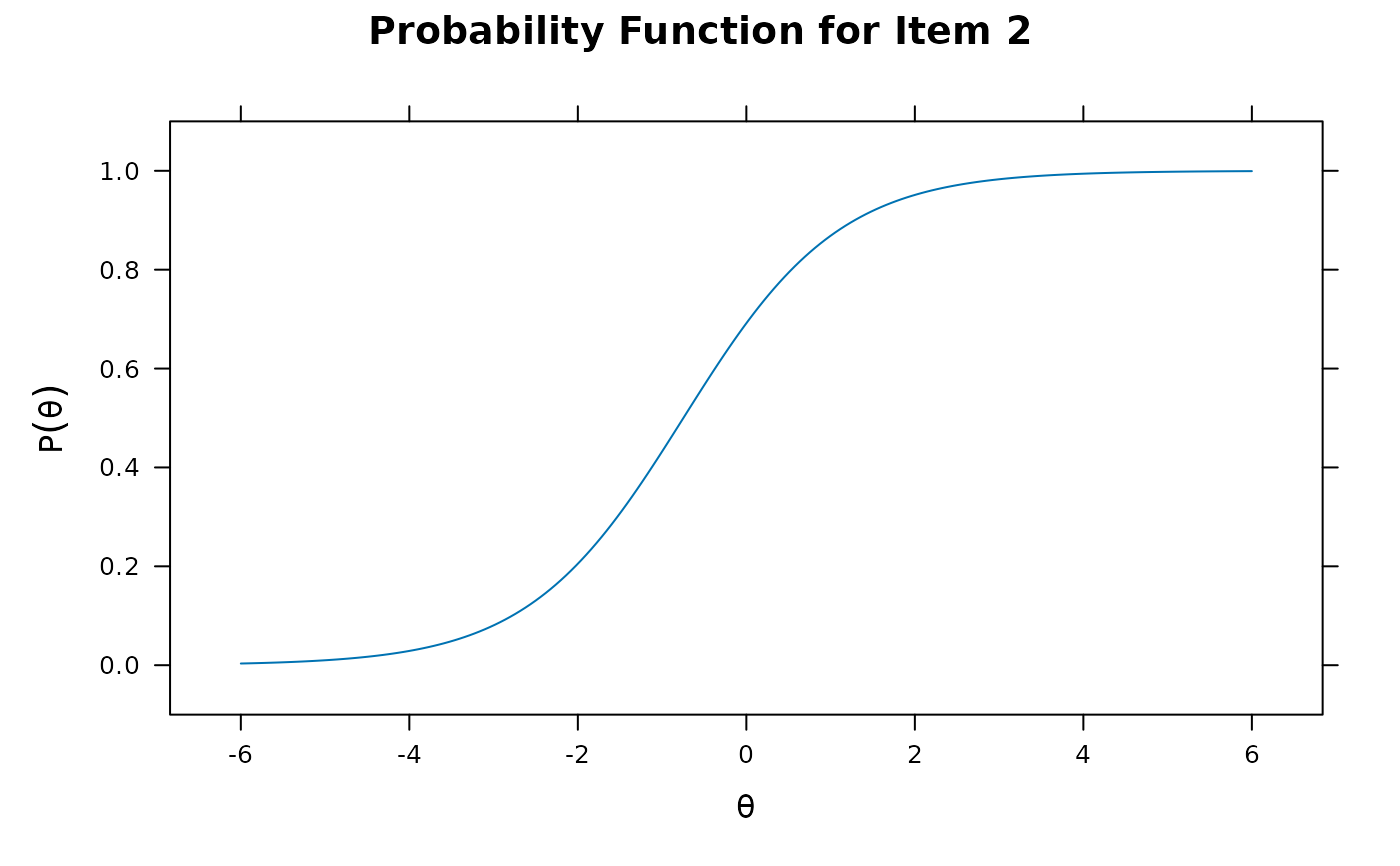
itemplot(mod1, 2)
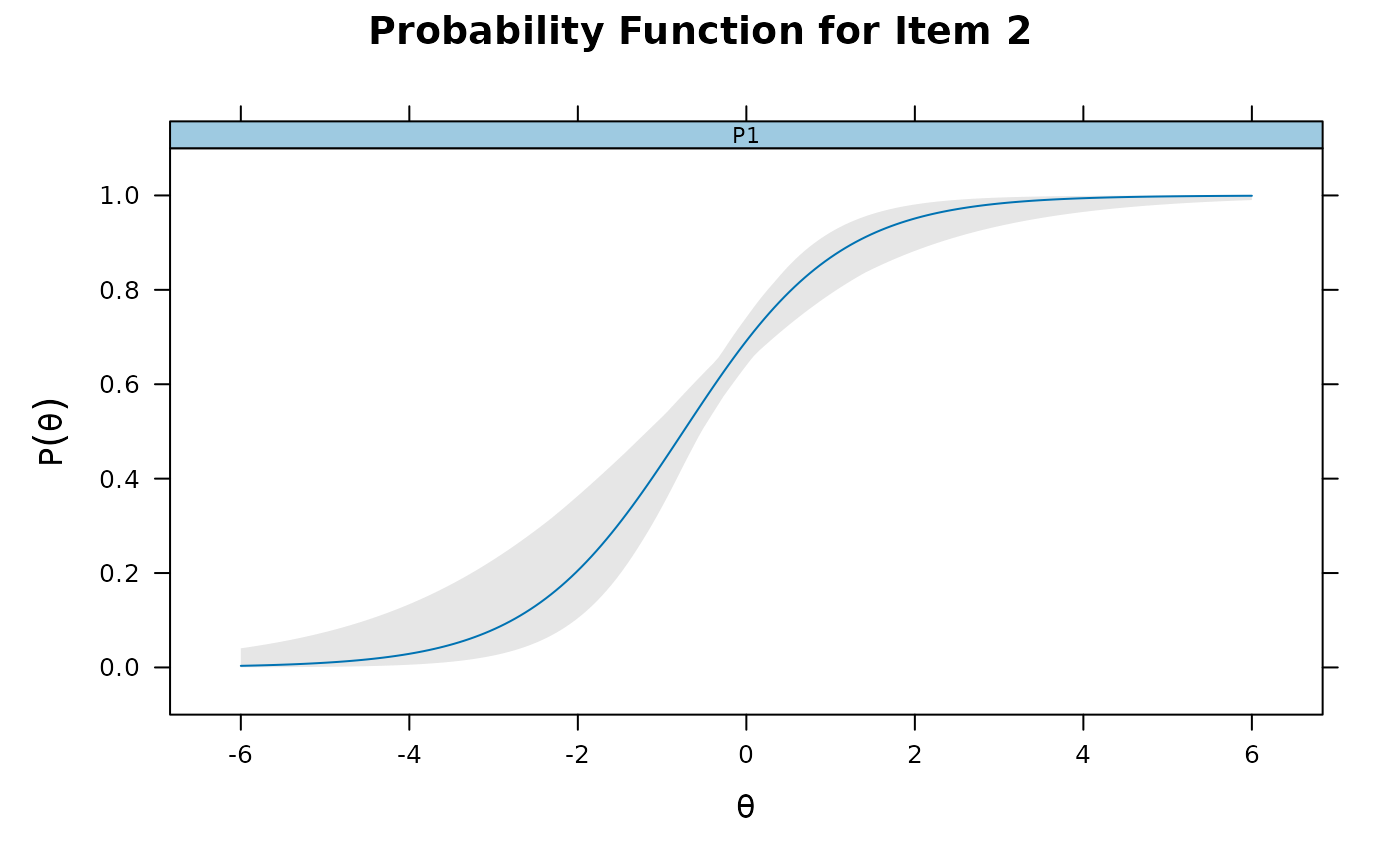
 itemplot(mod1, 2, CE = TRUE)
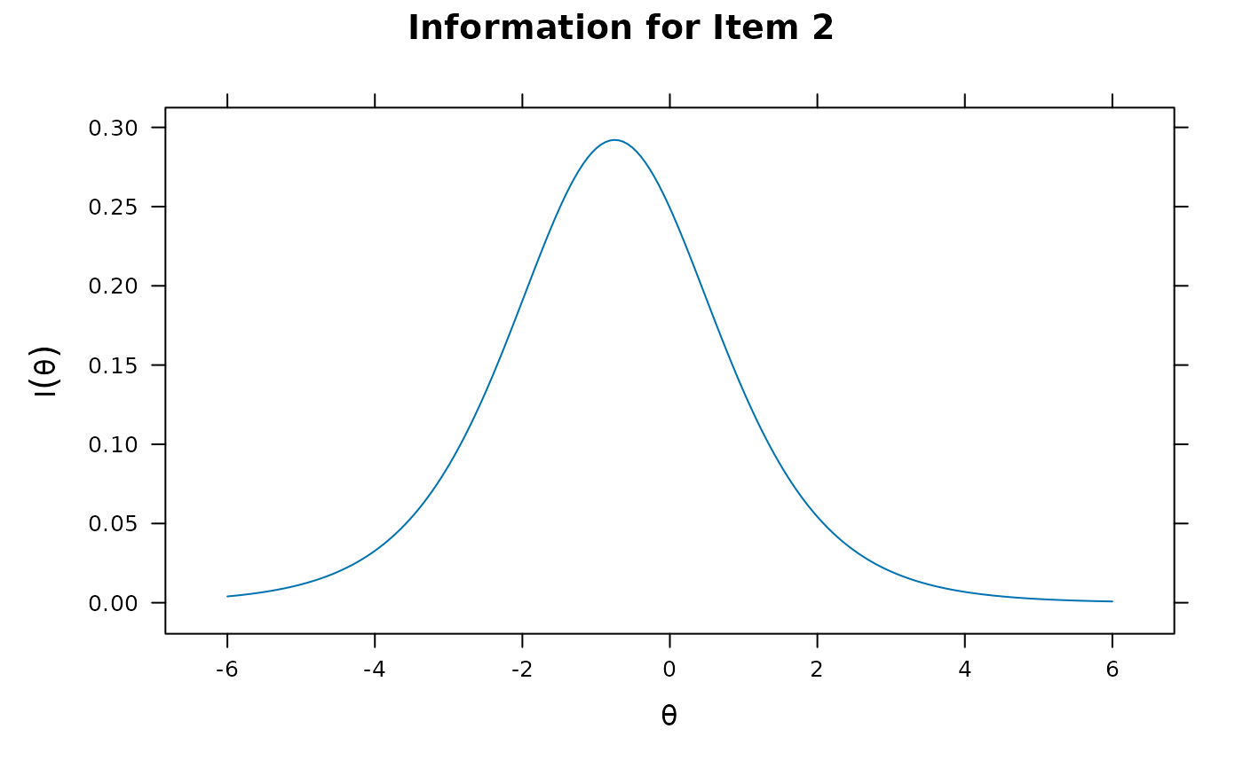
 itemplot(mod1, 2, type = 'info')
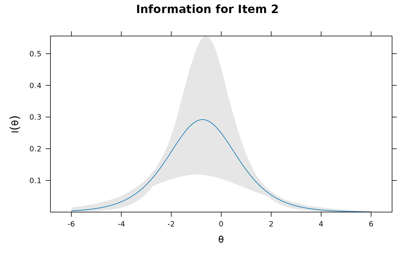
 itemplot(mod1, 2, type = 'info', CE = TRUE)
 mods <- list(twoPL = mod1, onePL = mod2)
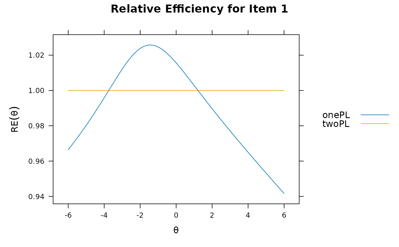
itemplot(mods, 1, type = 'RE')
mods <- list(twoPL = mod1, onePL = mod2)
itemplot(mods, 1, type = 'RE')
 # multidimensional
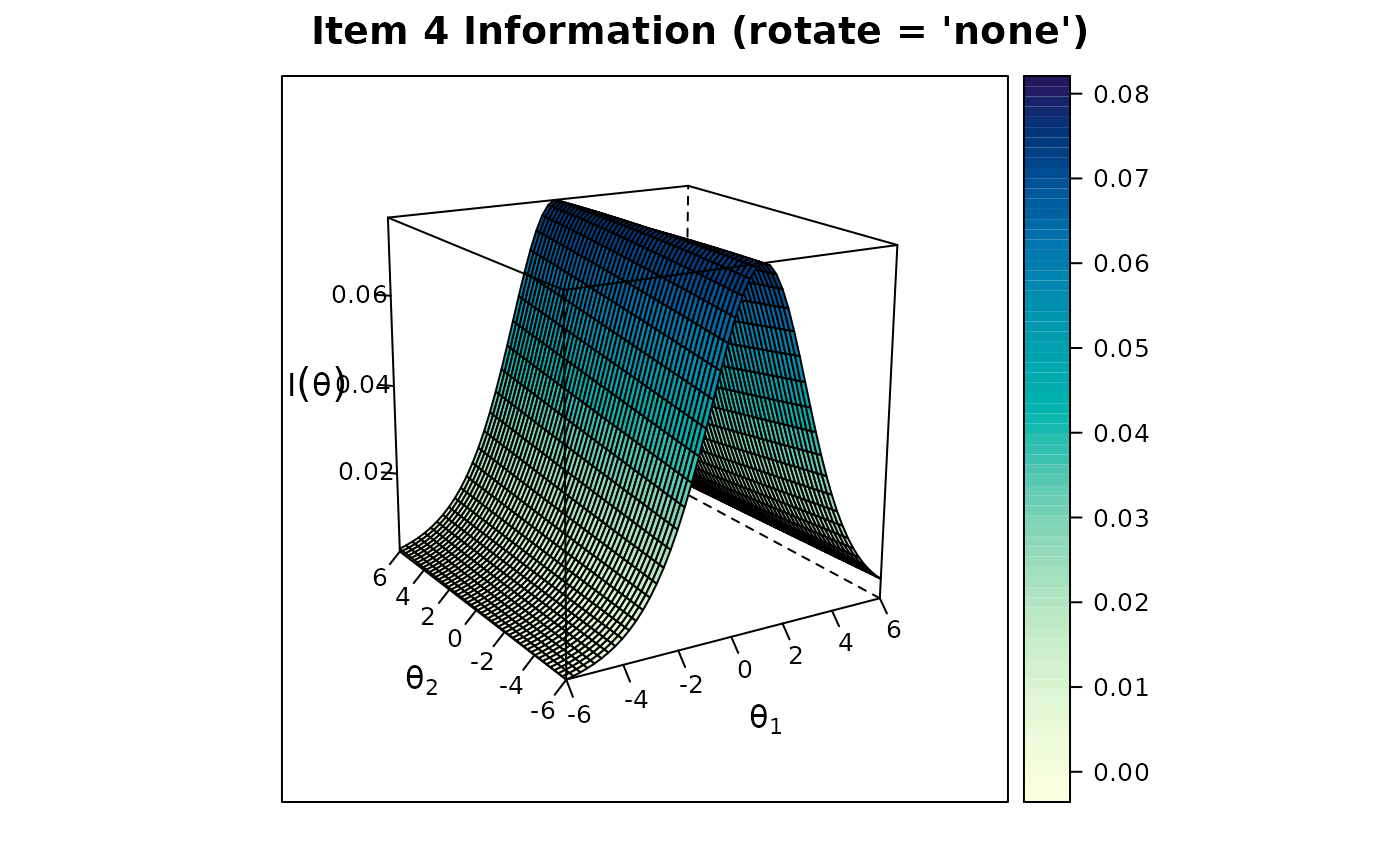
itemplot(mod3, 4, type = 'info')
# multidimensional
itemplot(mod3, 4, type = 'info')
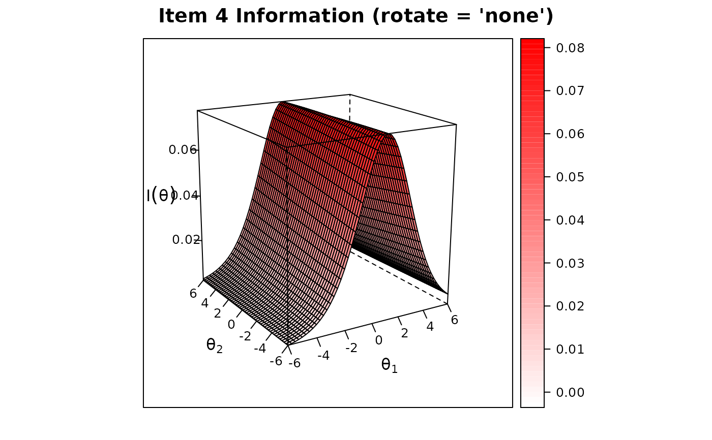
 itemplot(mod3, 4, type = 'info',
col.regions = colorRampPalette(c("white", "red"))(100))
itemplot(mod3, 4, type = 'info',
col.regions = colorRampPalette(c("white", "red"))(100))
 itemplot(mod3, 4, type = 'infocontour')
 itemplot(mod3, 4, type = 'tracecontour')
 # polytomous items
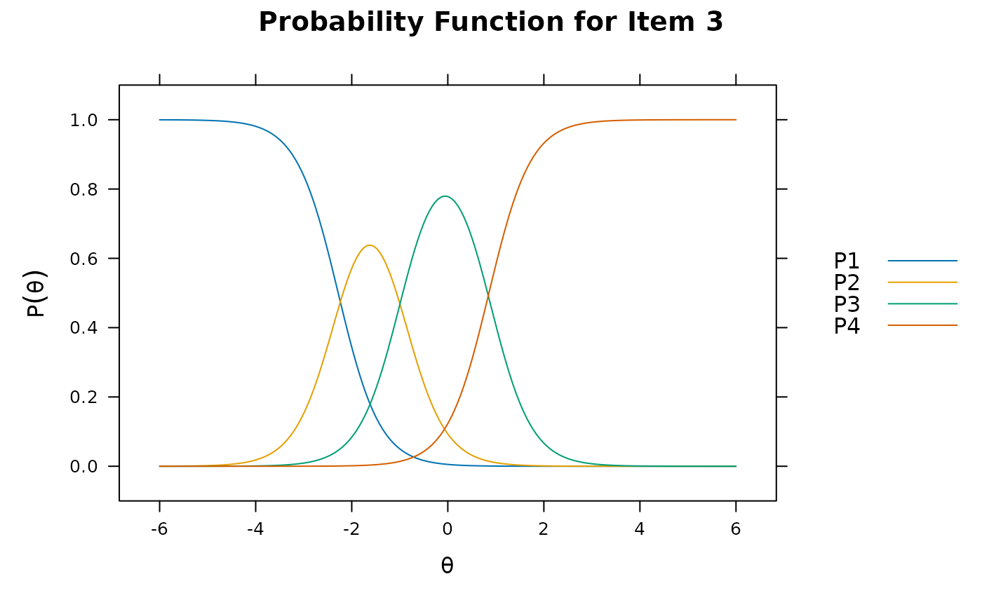
pmod <- mirt(Science, 1, SE=TRUE)
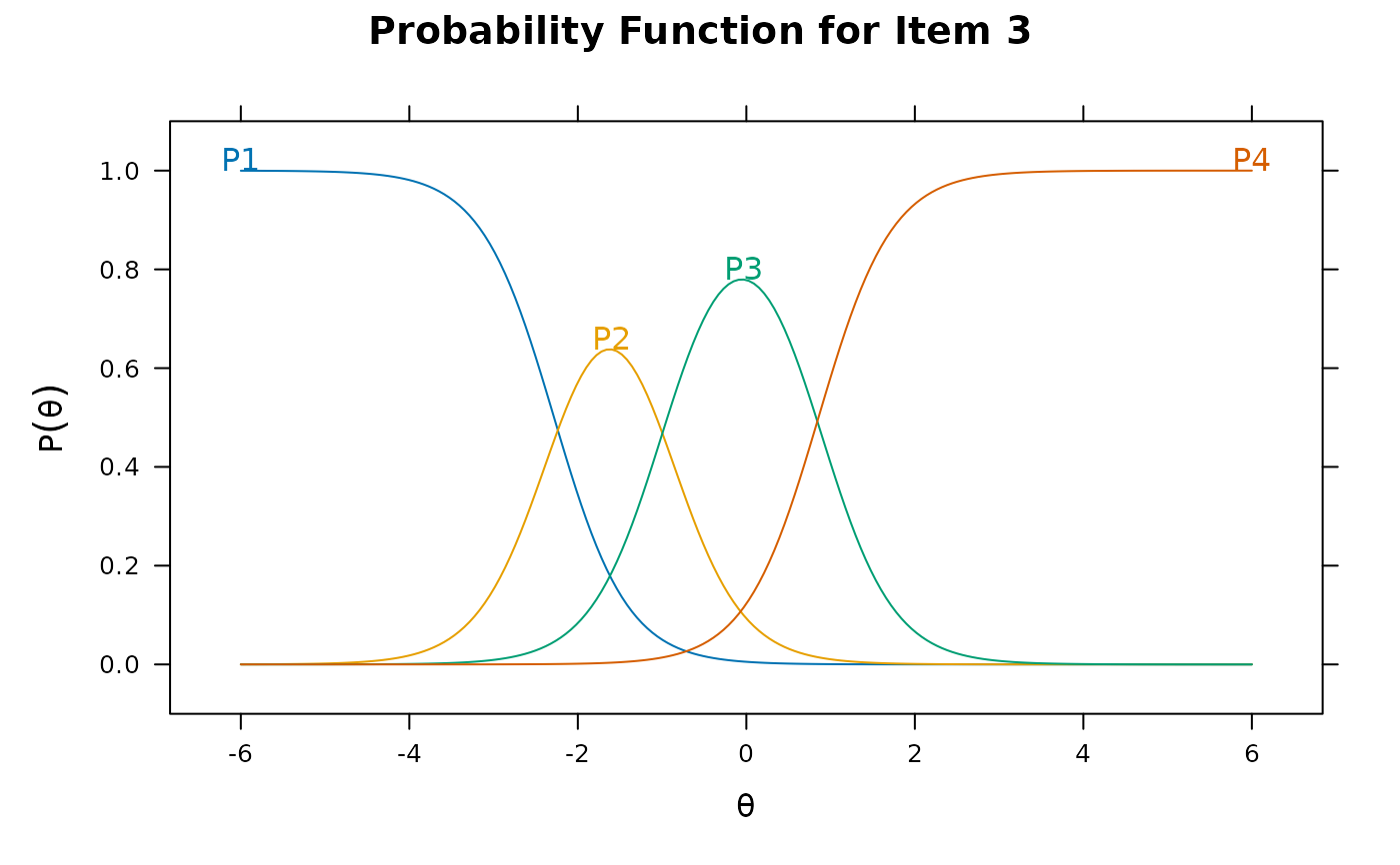
itemplot(pmod, 3)
# polytomous items
pmod <- mirt(Science, 1, SE=TRUE)
itemplot(pmod, 3)
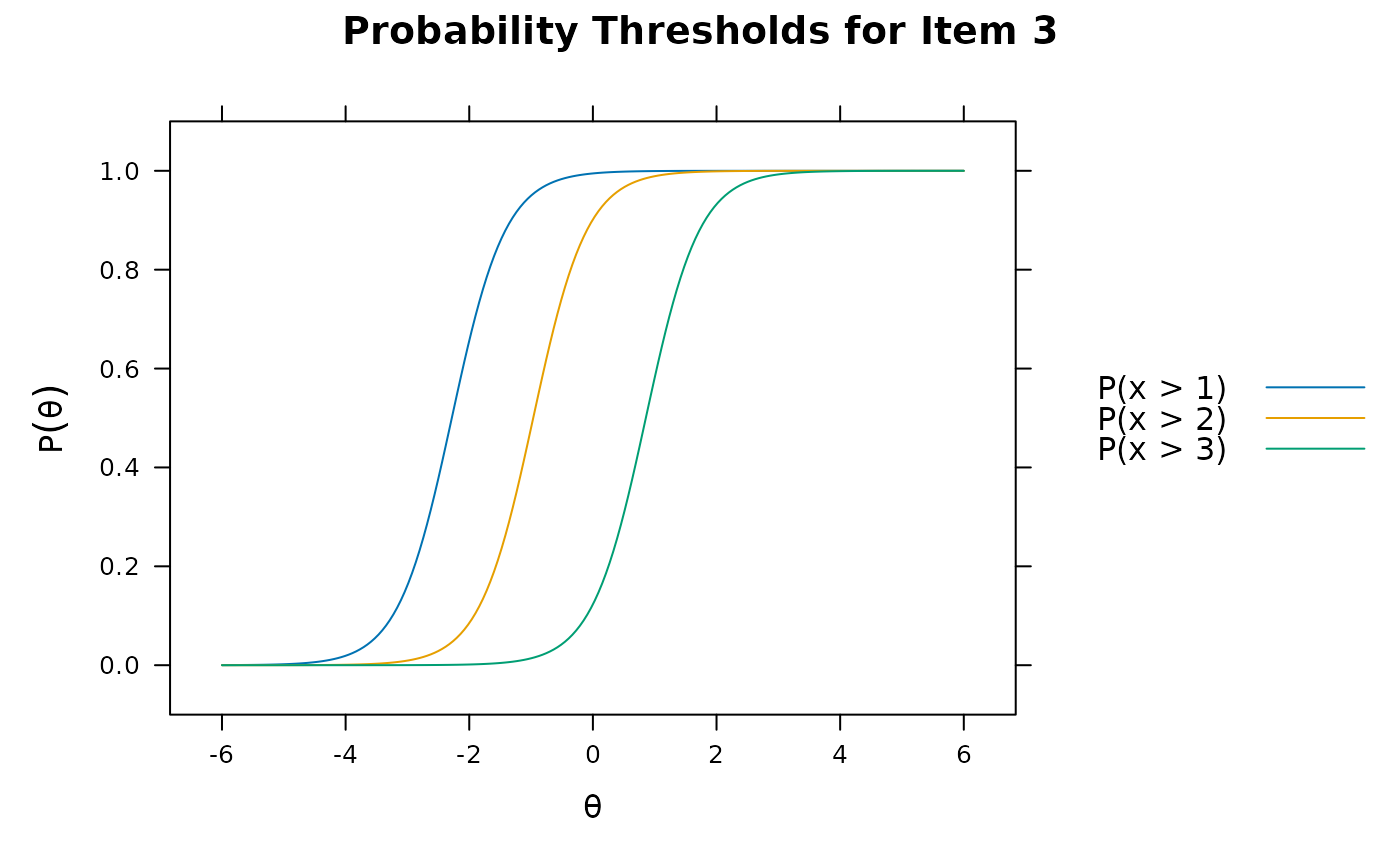
 itemplot(pmod, 3, type = 'threshold')
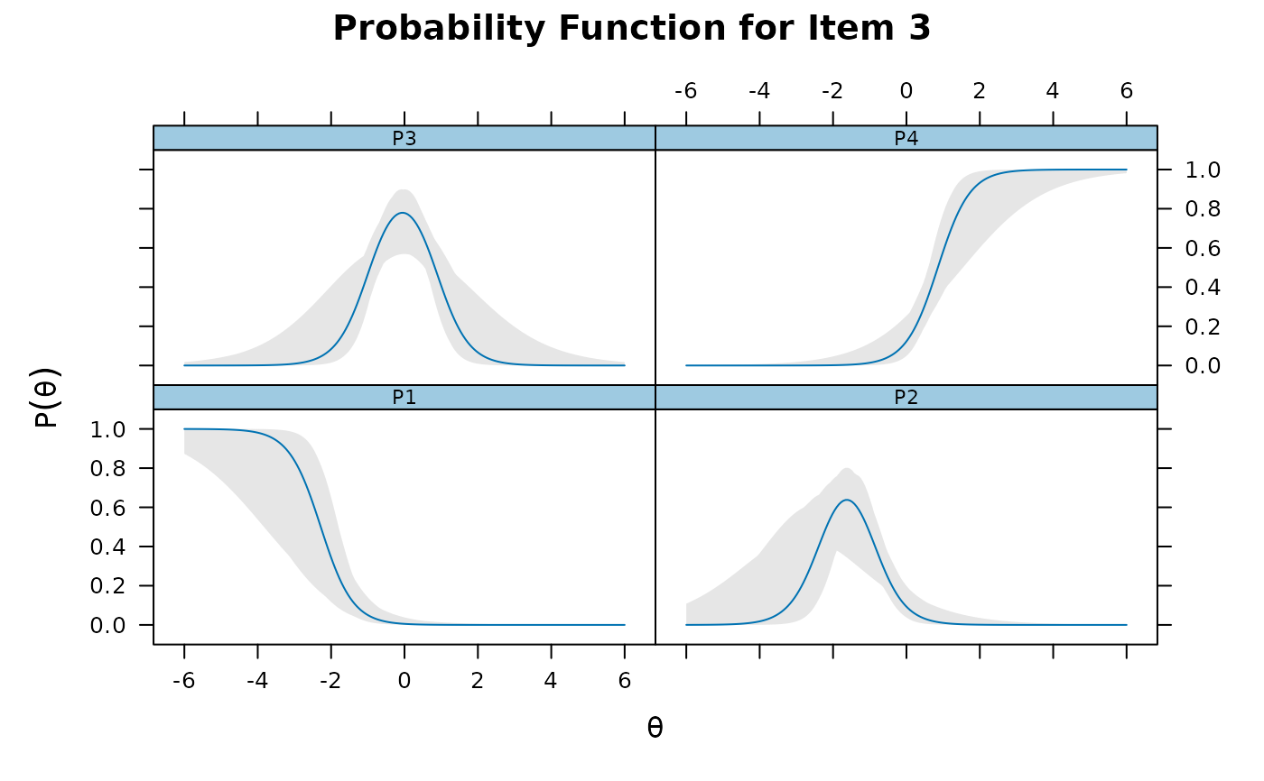
 itemplot(pmod, 3, CE = TRUE)
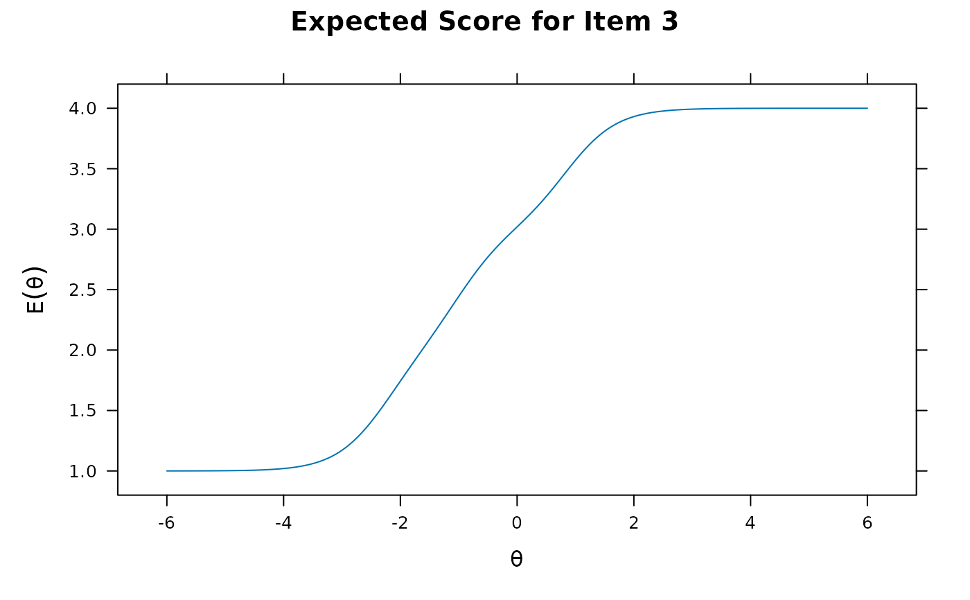
 itemplot(pmod, 3, type = 'score')
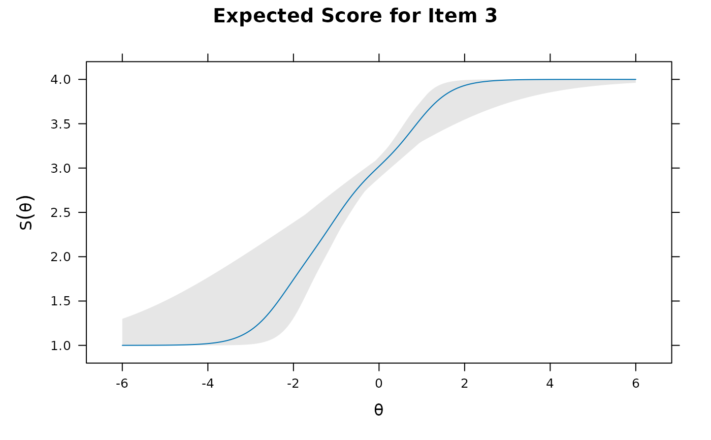
 itemplot(pmod, 3, type = 'score', CE = TRUE)
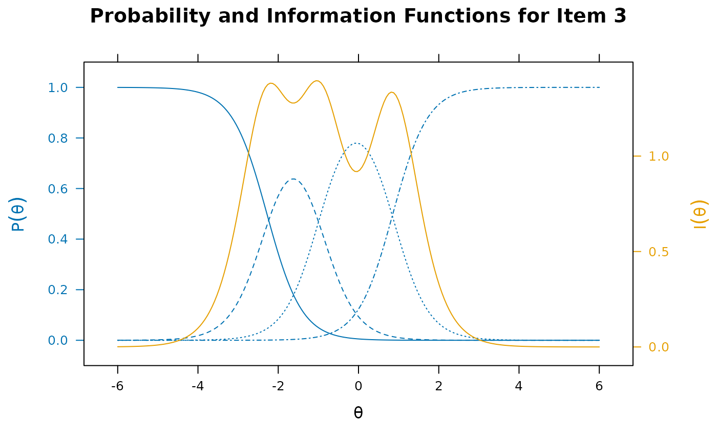
 itemplot(pmod, 3, type = 'infotrace')
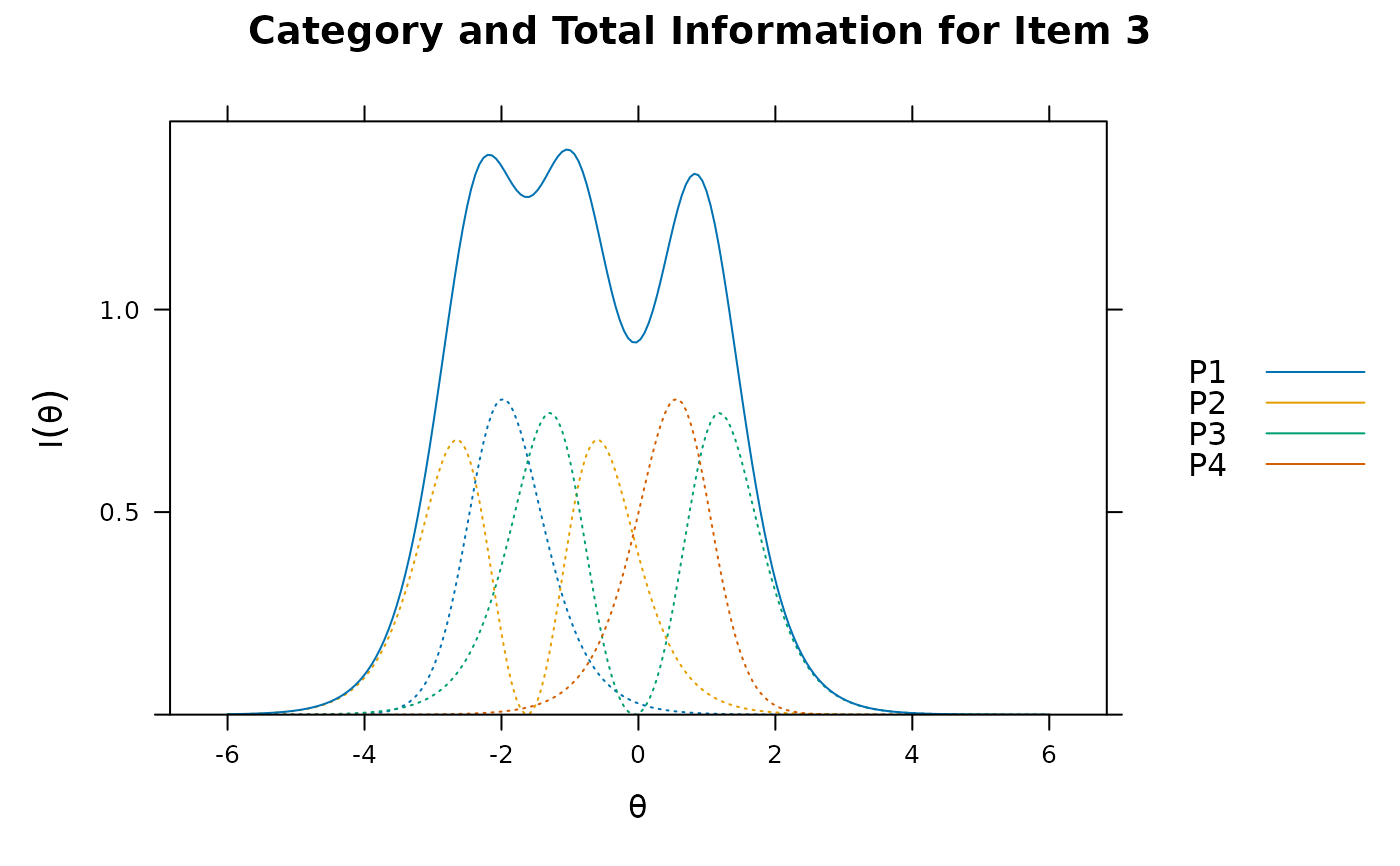
 itemplot(pmod, 3, type = 'infocat')
 # use the directlabels package to put labels on tracelines
library(directlabels)
plt <- itemplot(pmod, 3)
direct.label(plt, 'top.points')
# use the directlabels package to put labels on tracelines
library(directlabels)
plt <- itemplot(pmod, 3)
direct.label(plt, 'top.points')
 # change colour theme of plots
bwtheme <- standard.theme("pdf", color=FALSE)
plot(pmod, type='trace', par.settings=bwtheme)
# change colour theme of plots
bwtheme <- standard.theme("pdf", color=FALSE)
plot(pmod, type='trace', par.settings=bwtheme)
 itemplot(pmod, 1, type = 'trace', par.settings=bwtheme)
 # additional modifications can be made via update().
# See ?update.trellis for further documentation
(plt <- itemplot(pmod, 1))
# additional modifications can be made via update().
# See ?update.trellis for further documentation
(plt <- itemplot(pmod, 1))
 update(plt, ylab = expression(Prob(theta))) # ylab changed
 # infoSE plot
itemplot(pmod, 1, type = 'infoSE')
# infoSE plot
itemplot(pmod, 1, type = 'infoSE')
 # uncomment to run interactive shiny applet
# itemplot(shiny = TRUE)
# }
# uncomment to run interactive shiny applet
# itemplot(shiny = TRUE)
# }