Plot various test-implied functions from models

Plot various test implied response functions from models estimated in the mirt package.

# S4 method for MultipleGroupClass,missing
plot(
  x,
  y,
  type = "score",
  npts = 200,
  drop2 = TRUE,
  degrees = 45,
  which.items = 1:extract.mirt(x, "nitems"),
  rot = list(xaxis = -70, yaxis = 30, zaxis = 10),
  facet_items = TRUE,
  theta_lim = c(-6, 6),
  par.strip.text = list(cex = 0.7),
  par.settings = list(strip.background = list(col = "#9ECAE1"), strip.border = list(col =
    "black")),
  auto.key = list(space = "right", points = FALSE, lines = TRUE),
  ...
)

# S4 method for SingleGroupClass,missing
plot(
  x,
  y,
  type = "score",
  npts = 200,
  drop2 = TRUE,
  degrees = 45,
  theta_lim = c(-6, 6),
  which.items = 1:extract.mirt(x, "nitems"),
  MI = 0,
  CI = 0.95,
  rot = list(xaxis = -70, yaxis = 30, zaxis = 10),
  facet_items = TRUE,
  main = NULL,
  drape = TRUE,
  colorkey = TRUE,
  ehist.cut = 1e-10,
  add.ylab2 = TRUE,
  par.strip.text = list(cex = 0.7),
  par.settings = list(strip.background = list(col = "#9ECAE1"), strip.border = list(col =
    "black")),
  auto.key = list(space = "right", points = FALSE, lines = TRUE),
  profile = FALSE,
  ...
)

Arguments

x

an object of class SingleGroupClass, MultipleGroupClass, or DiscreteClass

y

an arbitrary missing argument required for R CMD check

type

type of plot to view. Can be

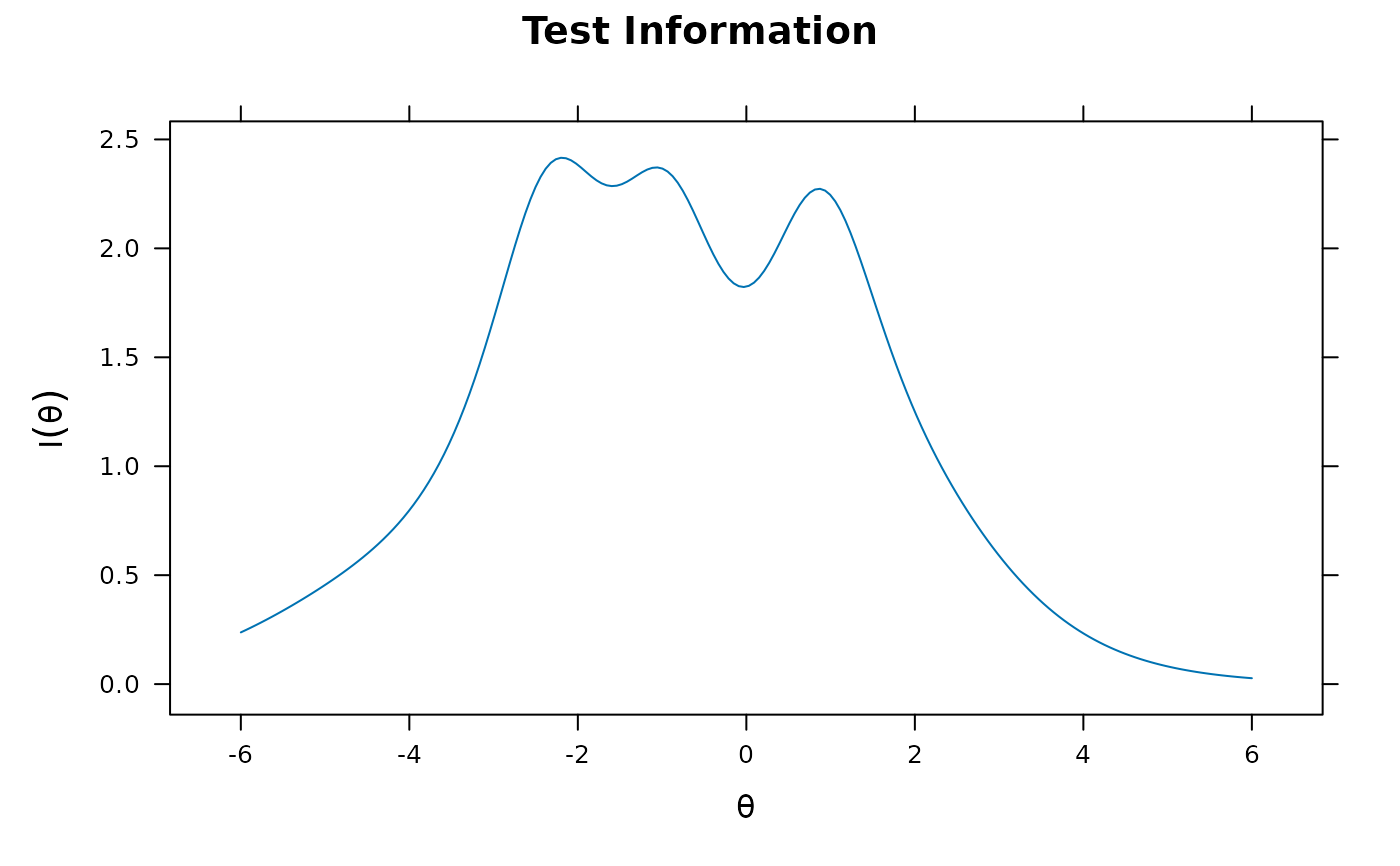
'info'

test information function

'rxx'

for the reliability function

'infocontour'

for the test information contours

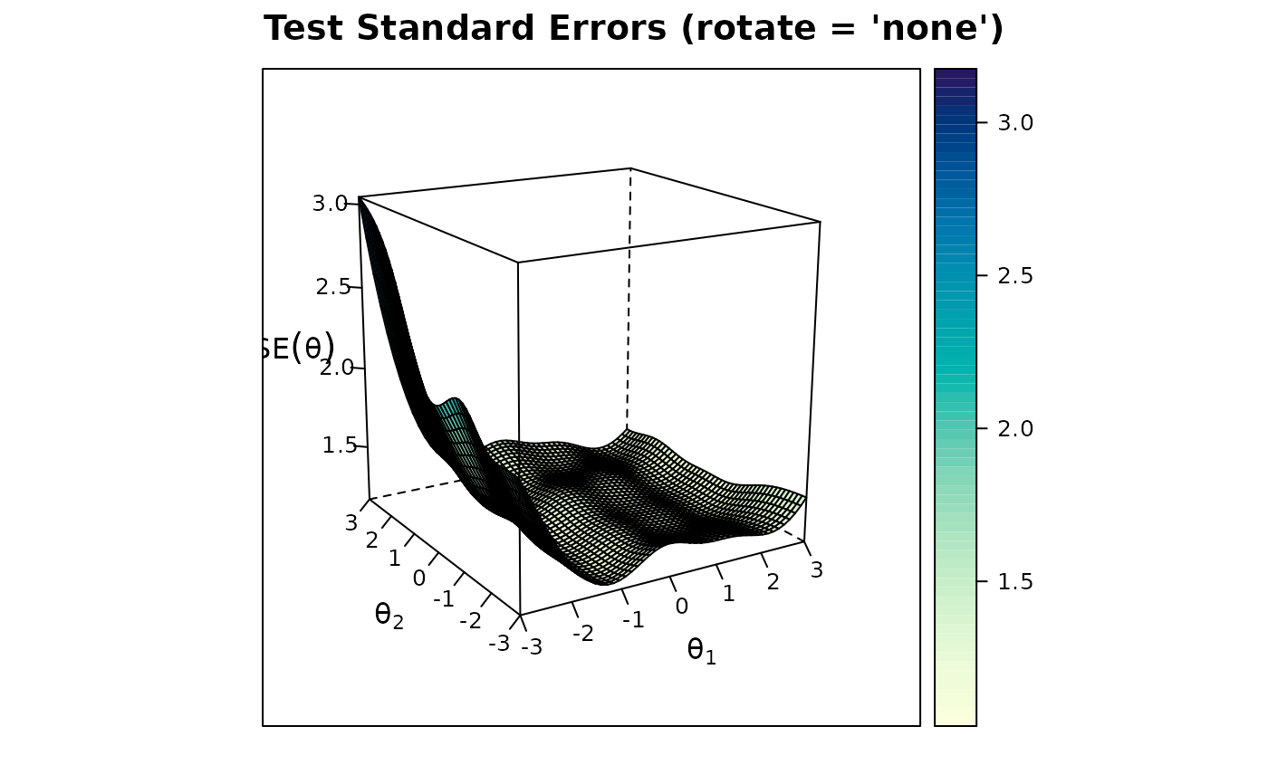
'SE'

for the test standard error function

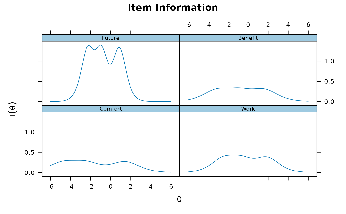
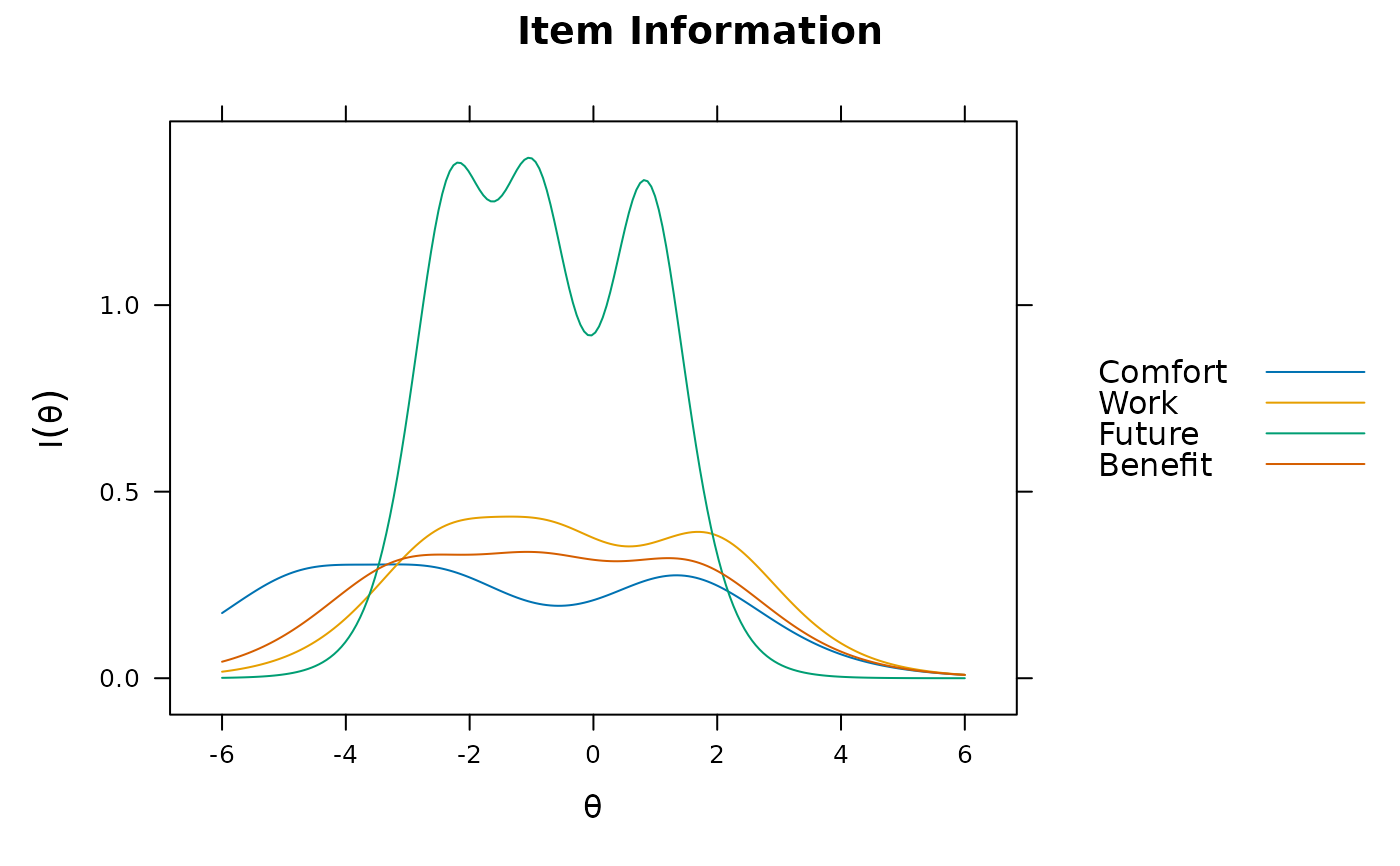
'infotrace'

item information traceline plots

'infoSE'

a combined test information and standard error plot

'trace'

item probability traceline plots

'itemscore'

item scoring traceline plots

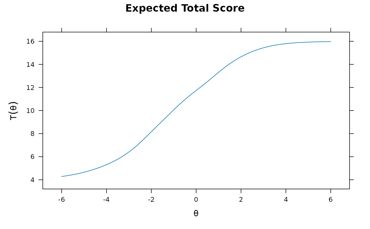
'score'

expected total score surface

'scorecontour'

expected total score contour plot

'posteriorTheta'

posterior for the latent trait distribution

'EAPsum'

compares sum-scores to the expected values based on the EAP for sum-scores method (see fscores)

Note that if dentype = 'empiricalhist' was used in estimation then the type 'empiricalhist' also will be available to generate the empirical histogram plot, and if dentype = 'Davidian-#' was used then the type 'Davidian' will also be available to generate the curve estimates at the quadrature nodes used during estimation

npts

number of quadrature points to be used for plotting features. Larger values make plots look smoother

drop2

logical; where appropriate, for dichotomous response items drop the lowest category and provide information pertaining only to the second response option?

degrees

numeric value ranging from 0 to 90 used in plot to compute angle for information-based plots with respect to the first dimension. If a vector is used then a bubble plot is created with the summed information across the angles specified (e.g., degrees = seq(0, 90, by=10))

which.items

numeric vector indicating which items to be used when plotting. Default is to use all available items

rot

allows rotation of the 3D graphics

facet_items

logical; apply grid of plots across items? If FALSE, items will be placed in one plot for each group

theta_lim

lower and upper limits of the latent trait (theta) to be evaluated, and is used in conjunction with npts

par.strip.text

plotting argument passed to lattice

par.settings

plotting argument passed to lattice

auto.key

plotting argument passed to lattice

...

additional arguments to be passed to lattice

MI

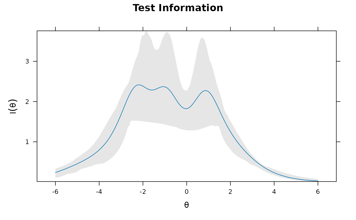
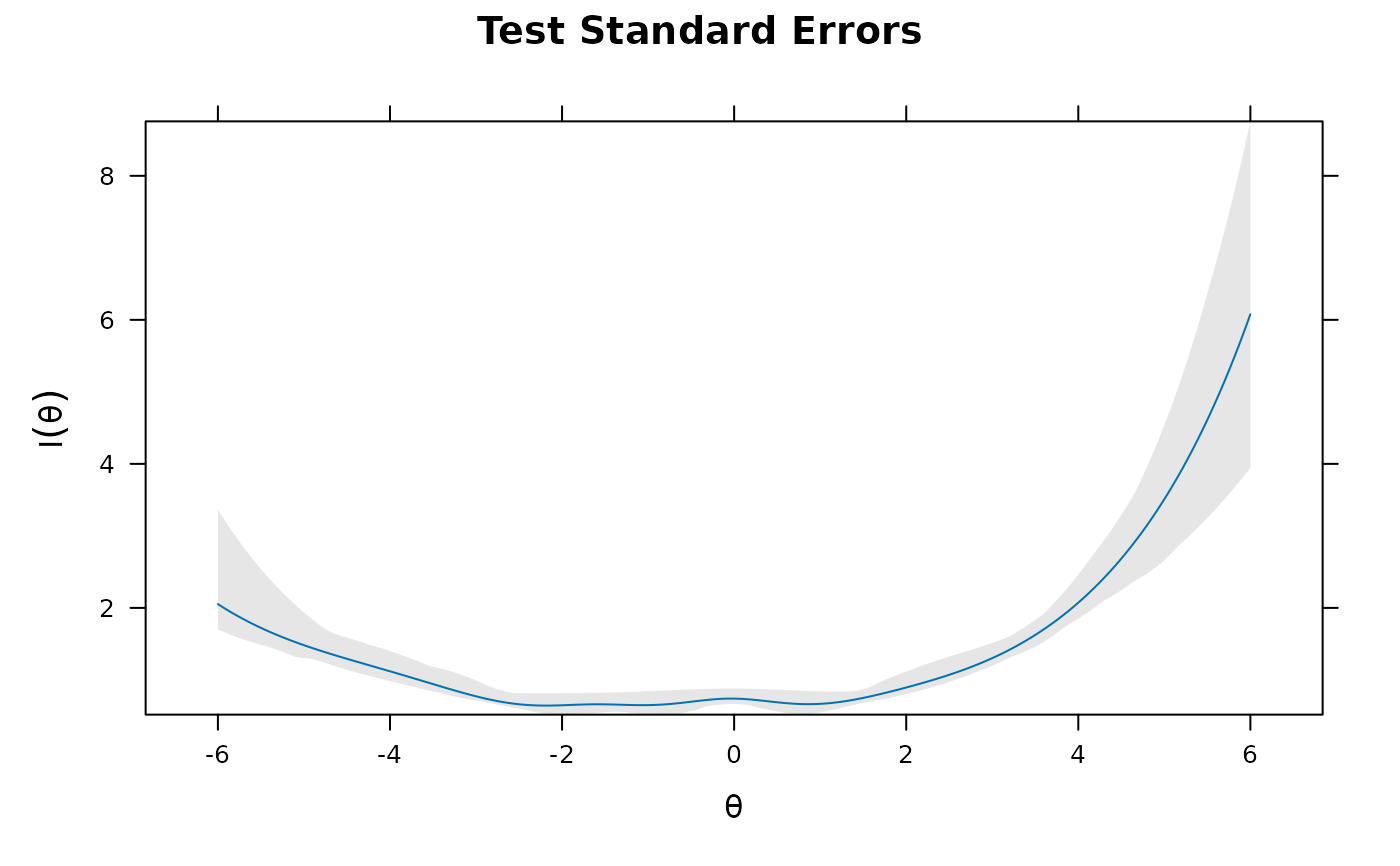
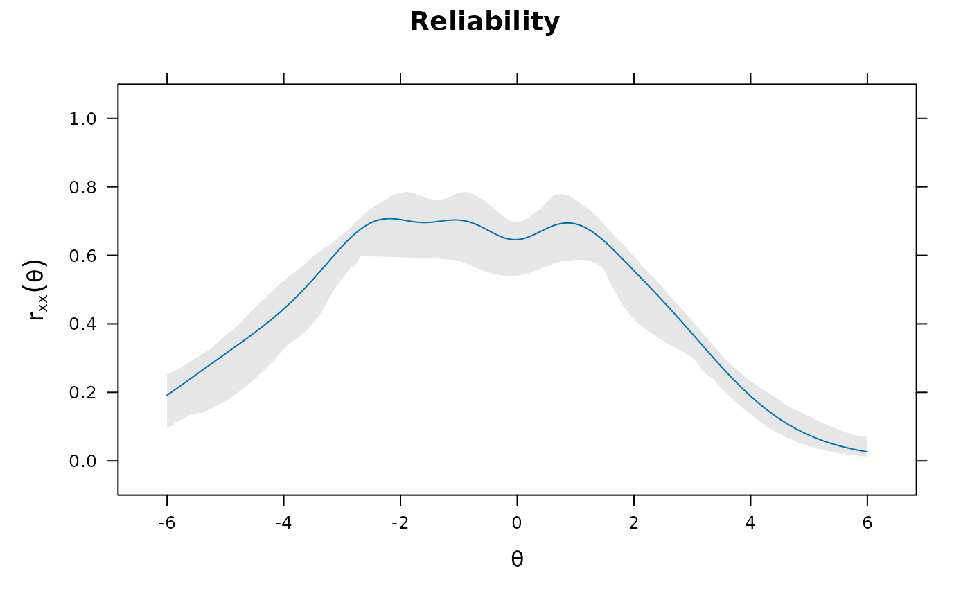
a single number indicating how many imputations to draw to form bootstrapped confidence intervals for the selected test statistic. If greater than 0 a plot will be drawn with a shaded region for the interval

CI

a number from 0 to 1 indicating the confidence interval to select when MI input is used. Default uses the 95% confidence (CI = .95)

main

argument passed to lattice. Default generated automatically

drape

logical argument passed to lattice. Default generated automatically

colorkey

logical argument passed to lattice. Default generated automatically

ehist.cut

a probability value indicating a threshold for excluding cases in empirical histogram plots. Values larger than the default will include more points in the tails of the plot, potentially squishing the 'meat' of the plot to take up less area than visually desired

add.ylab2

logical argument passed to lattice. Default generated automatically

profile

logical; provide a profile plot of response probabilities (objects returned from mdirt only)

References

Chalmers, R., P. (2012). mirt: A Multidimensional Item Response Theory Package for the R Environment. Journal of Statistical Software, 48(6), 1-29. doi:10.18637/jss.v048.i06

Examples

# \donttest{
x <- mirt(Science, 1, SE=TRUE)
plot(x)

plot(x, type = 'info')

plot(x, type = 'infotrace')

plot(x, type = 'infotrace', facet_items = FALSE)

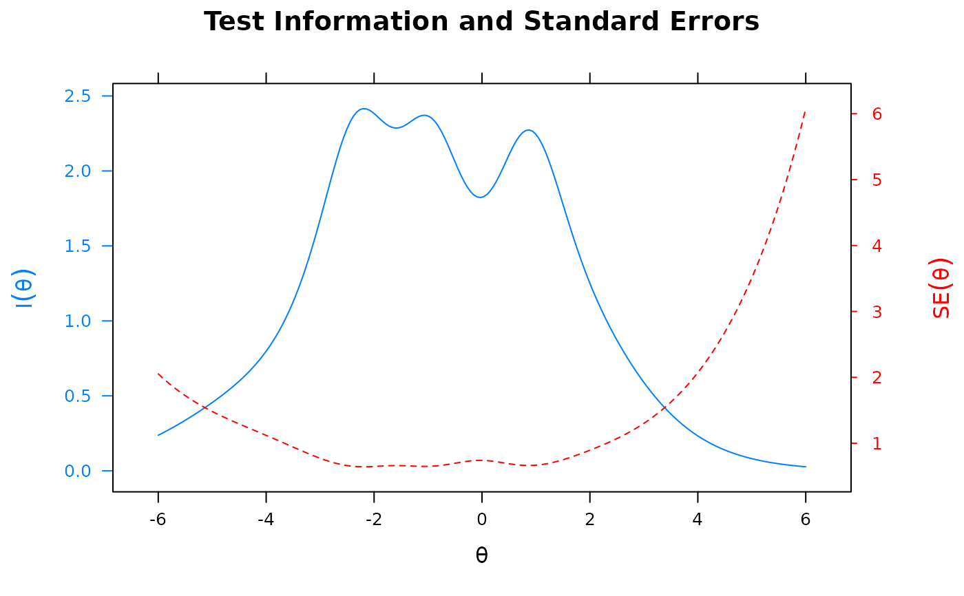
plot(x, type = 'infoSE')

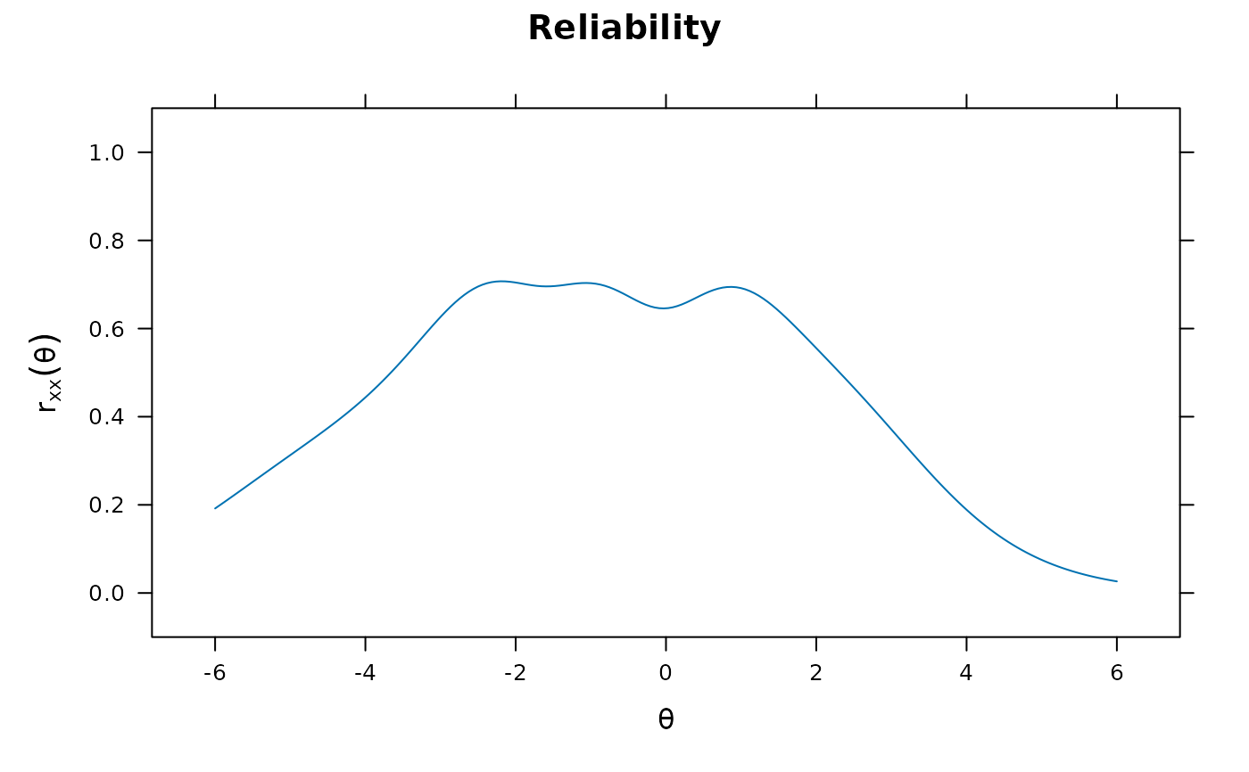
plot(x, type = 'rxx')

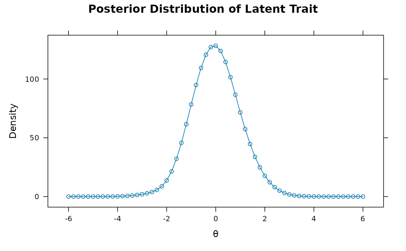
plot(x, type = 'posteriorTheta')


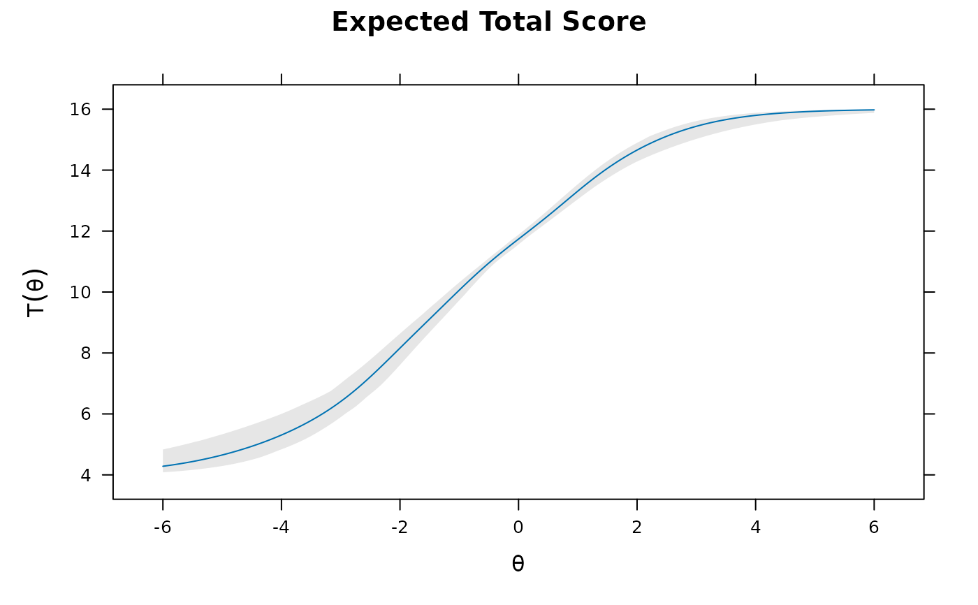
# confidence interval plots when information matrix computed
plot(x)

plot(x, MI=100)

plot(x, type='info', MI=100)

plot(x, type='SE', MI=100)

plot(x, type='rxx', MI=100)


# use the directlabels package to put labels on tracelines
library(directlabels)
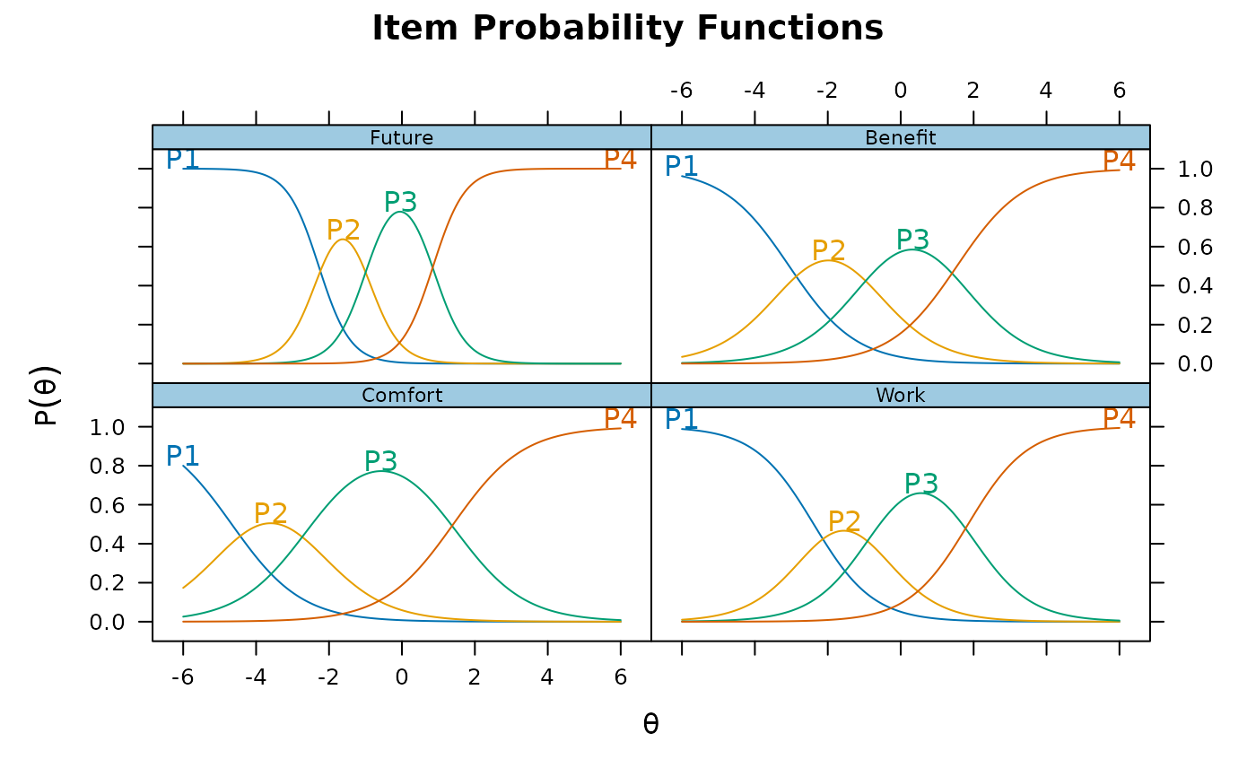
plt <- plot(x, type = 'trace')
direct.label(plt, 'top.points')


# additional modifications can be made via update().
# See ?update.trellis for further documentation
plt

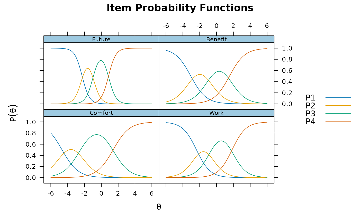update(plt, ylab = expression(Prob(theta)),
            main = "Item Traceline Functions") # ylab/main changed


set.seed(1234)
group <- sample(c('g1','g2'), nrow(Science), TRUE)
x2 <- multipleGroup(Science, 1, group)
plot(x2)

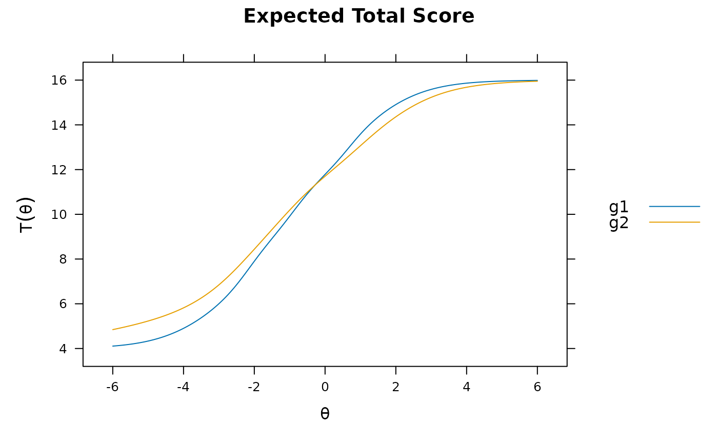plot(x2, type = 'trace')

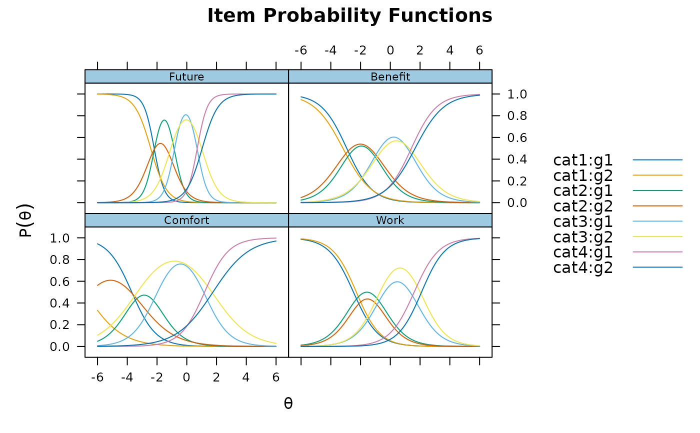plot(x2, type = 'trace', which.items = 1:2)

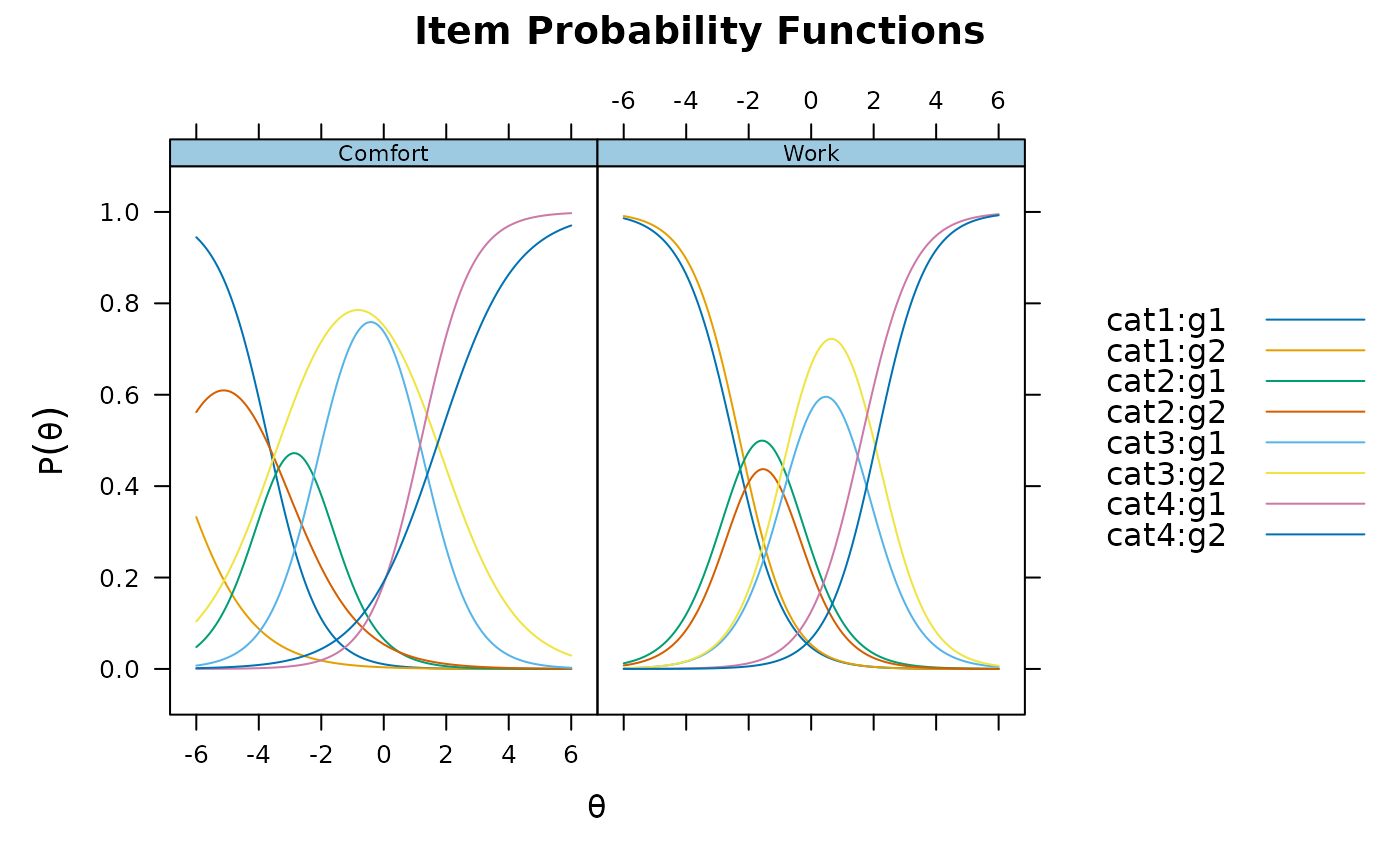plot(x2, type = 'itemscore', which.items = 1:2)

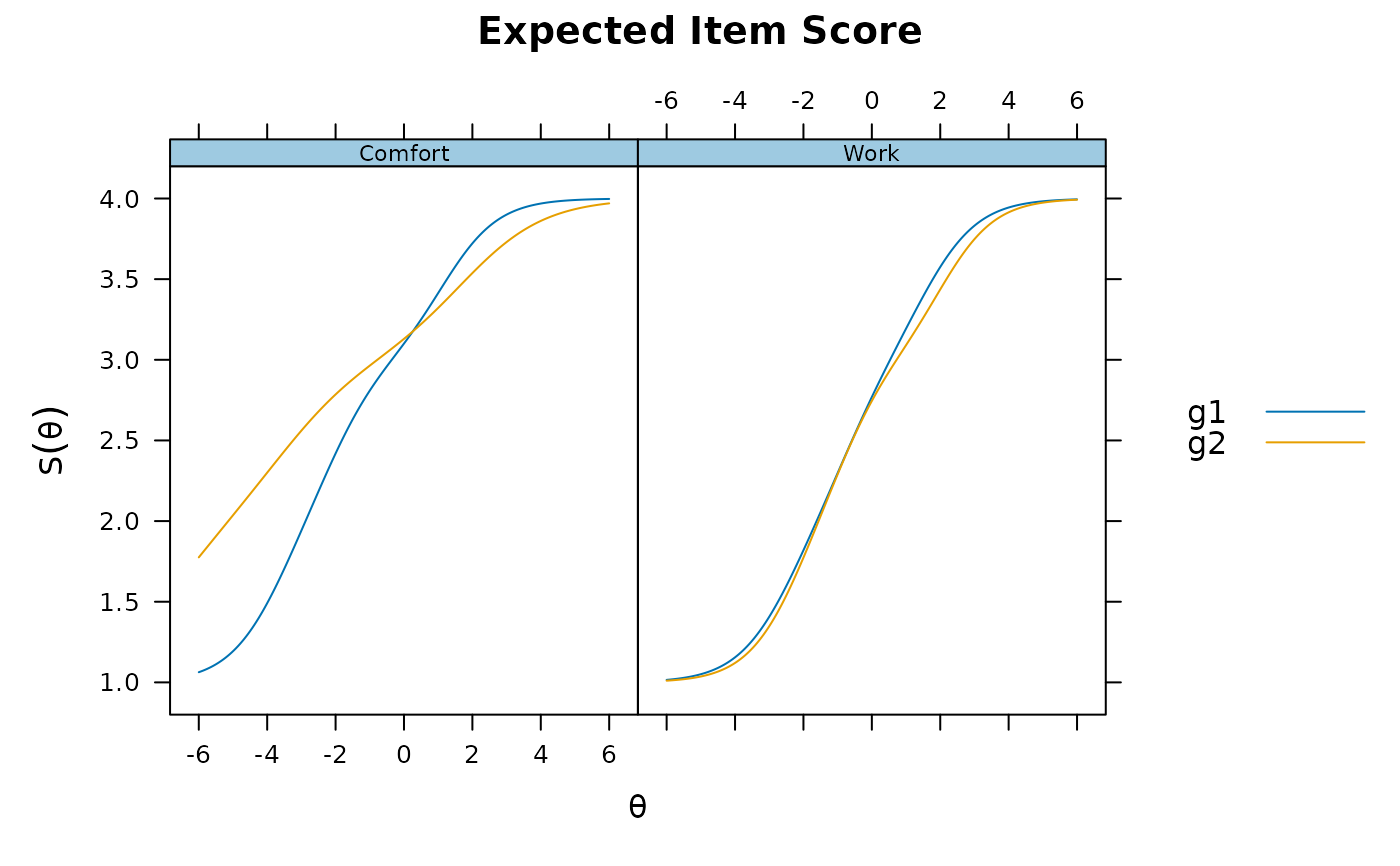plot(x2, type = 'trace', which.items = 1, facet_items = FALSE) #facet by group

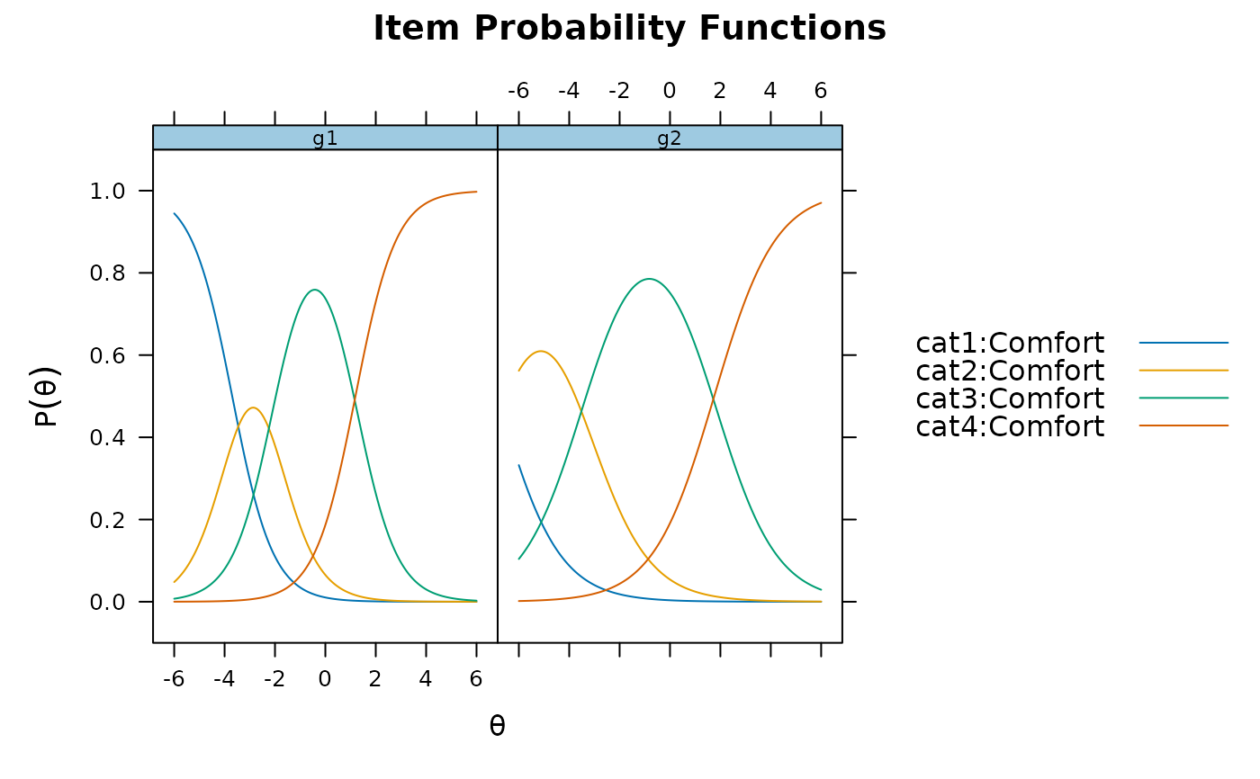plot(x2, type = 'info')


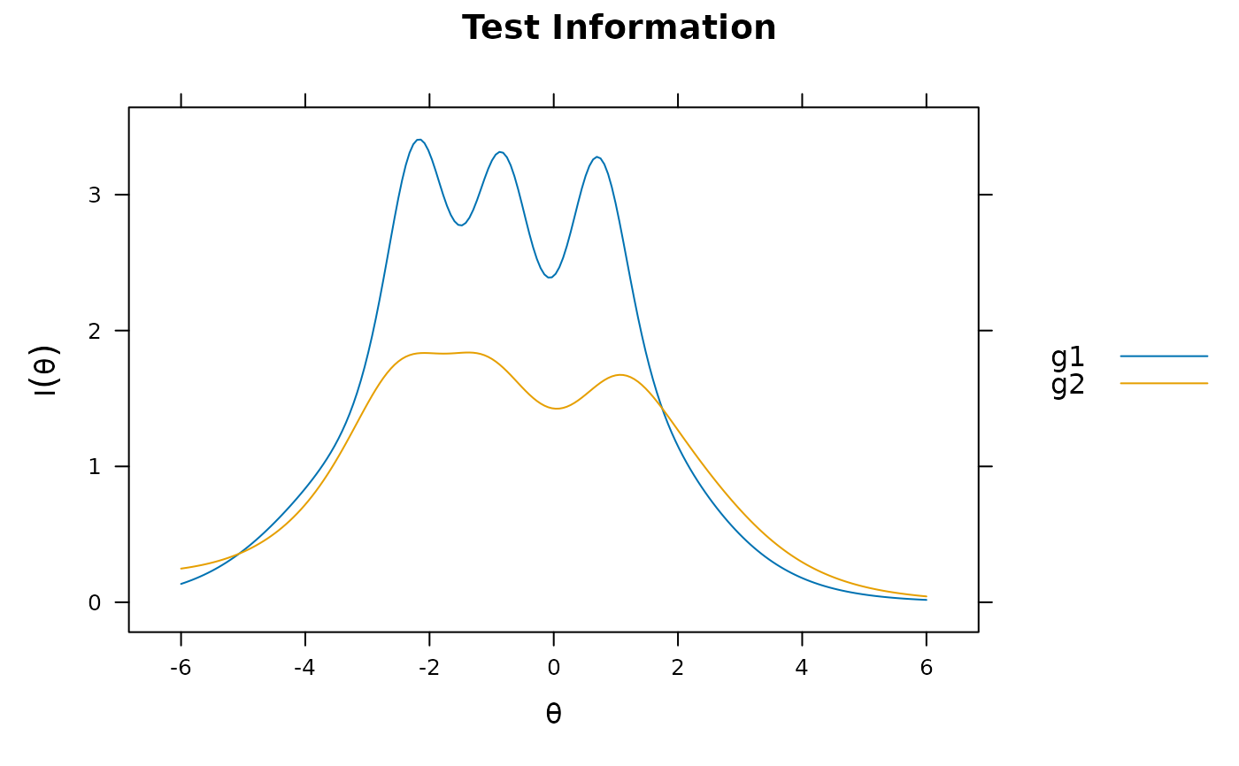x3 <- mirt(Science, 2)
plot(x3, type = 'info')

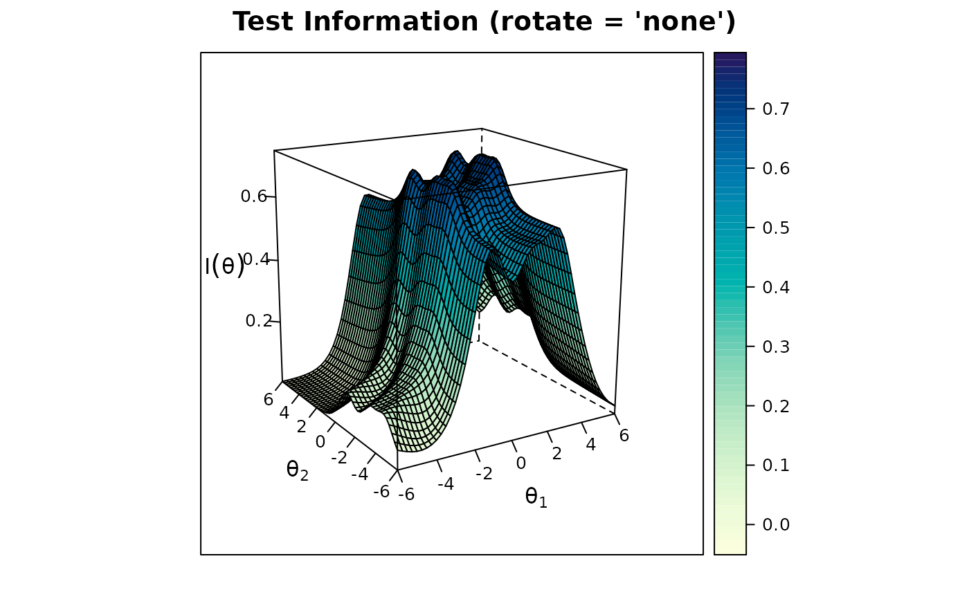plot(x3, type = 'SE', theta_lim = c(-3,3))


# }