Run a Monte Carlo simulation given conditions and simulation functions
Source:R/runSimulation.R
runSimulation.RdThis function runs a Monte Carlo simulation study given a set of predefined simulation functions,
design conditions, and number of replications. Results can be saved as temporary files in case of
interruptions and may be restored by re-running runSimulation, provided that the respective temp
file can be found in the working directory. runSimulation supports parallel
and cluster computing (with the parallel and
future packages; see also
runArraySimulation for submitting array jobs to HPC clusters),
global and local debugging, error handling (including fail-safe
stopping when functions fail too often, even across nodes), provides bootstrap estimates of the
sampling variability (optional), and automatic tracking of error and warning messages
with their associated .Random.seed states.
For convenience, all functions available in the R work-space are exported across all nodes
so that they are more easily accessible (however, other R objects are not, and therefore
must be passed to the fixed_objects input to become available across nodes).
Usage
runSimulation(
  design,
  replications,
  generate,
  analyse,
  summarise,
  prepare = NULL,
  fixed_objects = NULL,
  packages = NULL,
  filename = NULL,
  debug = "none",
  load_seed = NULL,
  load_seed_prepare = NULL,
  save = any(replications > 2),
  store_results = TRUE,
  save_results = FALSE,
  parallel = FALSE,
  ncores = parallelly::availableCores(omit = 1L),
  cl = NULL,
  notification = "none",
  notifier = NULL,
  beep = FALSE,
  sound = 1,
  check.globals = FALSE,
  CI = 0.95,
  seed = NULL,
  boot_method = "none",
  boot_draws = 1000L,
  max_errors = 50L,
  resume = TRUE,
  save_details = list(),
  control = list(),
  not_parallel = NULL,
  progress = TRUE,
  verbose = TRUE
)

# S3 method for class 'SimDesign'
summary(object, ...)

# S3 method for class 'SimDesign'
print(x, list2char = TRUE, ...)
Arguments
- design
a
tibbleordata.frameobject containing the Monte Carlo simulation conditions to be studied, where each row represents a unique condition and each column a factor to be varied. SeecreateDesignfor the standard approach to create this simulation design objectAs an augmentation of the input, the original
designobject can be passed toexpandDesignto systemically repeat the rows of each simulation condition, allowing smaller numbers ofreplicationsto be supplied per condition. After this distributed job is complete the functionSimCollectcan be used to recombine the results to a form commensurate with the originaldesignobject- replications
number of independent replications to perform per condition (i.e., each row in
design). Can be a single number, which will be used for each design condition, or an integer vector with length equal tonrow(design). All inputs must be greater than 0, though setting to less than 3 (for initial testing purpose) will disable thesaveandcontrol$stop_on_fatalflags- generate
user-defined data and parameter generating function (or named list of functions). See
Generatefor details. Note that this argument may be omitted by the user if they wish to generate the data with theanalysestep, but for real-world simulations this is generally not recommended. If multiple generate functions are provided as a list then the list of generate functions are executed in order until the first valid generate function is executed, where the subsequent generation functions are then ignored (seeGenerateIfto only apply data generation for specific conditions).- analyse
user-defined analysis function (or named list of functions) that acts on the data generated from
Generate(or, ifgeneratewas omitted, can be used to generate and analyse the simulated data). SeeAnalysefor details- summarise
optional (but strongly recommended) user-defined summary function from
Summariseto be used to compute meta-statistical summary information after all the replications have completed within eachdesigncondition. Return of this function, in order of increasing complexity, should be: a named numeric vector ordata.framewith one row, amatrixordata.framewith more than one row, and, failing these more atomic types, a namedlist. When alistis returned the final simulation object will contain a columnSUMMARISEcontaining the summary results for each respective conditionNote that unlike the Generate and Analyse steps, the Summarise portion is not as important to perfectly organize as the results can be summarised later on by using the built-in
reSummarisefunction (provided eitherstore_results = TRUEorsave_results = TRUEwere included).Omitting this function will return a tibble with the
Designand associated results information for allnrow(Design) * replicationsevaluations if the results from eachAnalyse()call was a one-dimensional vector. For more general objects returned byAnalyse()(such aslists), alistcontaining the results returned fromAnalyse. This is generally only recommended for didactic purposes because the results will leave out a large amount of information (e.g., try-errors, warning messages, saving files, etc), can witness memory related issues if the Analyse function returns larger objects, and generally is not as flexible internally. However, it may be useful when replications are expensive and ANOVA-based decompositions involving the within-condition replication information are of interest, though of course this can be circumvented by usingstore_results = TRUEorsave_results = TRUEwith or without a suppliedsummarisedefinition.Finally, there are keywords that should not be returned from this function, since they will cause a conflict with the aggregated simulation objects. These are currently those listed in capital letters (e.g.,
ERRORS,WARNINGS,REPLICATIONS, etc), all of which can be avoided if the returned objects are not entirely capitalized (e.g.,Errors,errors,ErRoRs, ..., will all avoid conflicts)- prepare
(optional) a function that executes once per simulation condition (i.e., once per row in
design) to load or prepare condition-specific objects intofixed_objectsbefore replications are run. This function should acceptconditionandfixed_objectsas arguments and return the modifiedfixed_objects.The primary use case is to load pre-computed objects from disk that were generated offline:
prepare <- function(condition, fixed_objects) {# Create filename from design parametersfname <- paste0('prepare/N', condition$N, '_SD', condition$SD, '.rds')fixed_objects$expensive_stuff <- readRDS(fname)fixed_objects}This approach allows you to: (1) pre-generate expensive condition-specific objects prior to running the simulation, (2) save them as individual RDS files, and (3) load them efficiently during the simulation. This is preferable to generating objects within
prepare()itself because it allows you to inspect the objects, ensures reproducibility, and separates object generation from the simulation workflow.Note: Objects added to
fixed_objectsinprepare()are not stored byrunSimulation()to conserve memory, as they are typically large. You should maintain your own records of these objects outside the simulation.RNG Warning: If you generate objects within
prepare()using random number generation (e.g.,rnorm(),runif()), reproducibility requires explicit RNG state management viastore_Random.seeds=TRUEandload_seed_prepare. Pre-computing and saving objects as RDS files is the recommended approach for reproducible simulations.The function signature should be:
prepare <- function(condition, fixed_objects) { ... return(fixed_objects) }Default is
NULL, in which case no preparation step is performed- fixed_objects
(optional) an object (usually a named
list) containing additional user-defined objects that should remain fixed across conditions. This is useful when including large vectors/matrices of population parameters, fixed data information that should be used across all conditions and replications (e.g., including a common design matrix for linear regression models), or simply control constant global elements (e.g., a constant for sample size)- packages
a character vector of external packages to be used during the simulation (e.g.,
c('MASS', 'extraDistr', 'simsem')), though if a logical operator is detected will be passed toCheckPackagesas well to ensure that the strong package version dependencies are verified before executing the code (e.g.,c('MASS >= 7.3.65', 'extraDistr == 1.10.0.4')).Use this input when running code in parallel to use non-standard functions from additional packages. Note that any previously attached packages explicitly loaded via
libraryorrequirewill be automatically added to this list, provided that they are visible in theotherPkgselement fromsessionInfo. Alternatively, functions can be called explicitly without attaching the package with the::operator (e.g.,extraDistr::rgumbel())- filename
(optional) the name of the
.rdsfile to save the final simulation results to. If the extension.rdsis not included in the file name (e.g."mysimulation"versus"mysimulation.rds") then the.rdsextension will be automatically added to the file name to ensure the file extension is correct.Note that if the same file name already exists in the working directly at the time of saving then a new file will be generated instead and a warning will be thrown. This helps to avoid accidentally overwriting existing files. Default is
NULL, indicating no file will be saved by default- debug
a string indicating where to initiate a
browser()call for editing and debugging, and pairs particularly well with theload_seedargument for precise debugging. General options are'none'(default; no debugging),'error', which starts the debugger when any error in the code is detected in one of three generate-analyse-summarise functions, and'all', which debugs all the user defined functions regardless of whether an error was thrown or not. Specific options include:'generate'to debug the data simulation function,'analyse'to debug the computational function, and'summarise'to debug the aggregation function.If the
Analyseargument is supplied as a named list of functions then it is also possible to debug the specific function of interest by passing the name of the respective function in the list. For instance, ifanalyse = list(A1=Analyse.A1, A2=Analyse.A2)then passingdebug = 'A1'will debug only the first function in this list, and all remaining analysis functions will be ignored.For debugging specific rows in the
Designinput (e.g., when a number of initial rows successfully complete but thekth row fails) the row number can be appended to the standarddebuginput using a'-'separator. For instance, debugging whenever an error is raised in the second row ofDesigncan be declared viadebug = 'error-2'.Finally, users may place
browsercalls within the respective functions for debugging at specific lines, which is useful when debugging based on conditional evaluations (e.g.,if(this == 'problem') browser()). Note that parallel computation flags will automatically be disabled when abrowser()is detected or when a debugging argument other than'none'is supplied- load_seed
used to replicate an exact simulation state, which is primarily useful for debugging purposes. Input can be a character object indicating which file to load from when the
.Random.seeds have be saved (after a call withsave_seeds = TRUE), or an integer vector indicating the actual.Random.seedvalues (e.g., extracted after usingstore_seeds). E.g.,load_seed = 'design-row-2/seed-1'will load the first seed in the second row of thedesigninput, or explicitly passing the elements from.Random.seed(seeSimExtractorSimErrorsto extract the seeds associated explicitly with errors during the simulation, where each column represents a unique seed). If the input is a character vector then it is important NOT to modify thedesigninput object, otherwise the path may not point to the correct saved location, while if the input is an integer vector (or single columntblobject) then it WILL be important to modify thedesigninput in order to load this exact seed for the corresponding design row. Default isNULL- load_seed_prepare
similar to
load_seed, but specifically for debugging thepreparefunction. Used to replicate the exact RNG state when prepare is called for a given condition. Accepts the same input formats asload_seed: a character string path (e.g.,'design-row-2/prepare-seed'), an integer vector containing the.Random.seedstate, or a tibble/data.frame with seed values. This is particularly useful when prepare encounters an error and you need to reproduce the exact state. The prepare error seed can be extracted usingSimExtract(res, 'prepare_error_seed'). Default isNULL- save
logical; save the temporary simulation state to the hard-drive using
qs2::qd_save()? This is useful for simulations which require an extended amount of time, though for shorter simulations can be disabled to slightly improve computational efficiency. WhenTRUE, which is the default when evaluatingreplications > 2, a temp file will be created in the working directory which allows the simulation state to be saved and recovered (in case of power outages, crashes, etc). As well, triggering this flag will save any fatal.Random.seedstates when conditions unexpectedly crash (where each seed is stored row-wise in an external .rds file), which provides a much easier mechanism to debug issues (seeload_seedfor details). Upon completion, this temp file will be removed.To recover your simulation at the last known location (having patched the issues in the previous execution code) simply re-run the code you used to initially define the simulation and the external file will automatically be detected and read-in. Default is
TRUEwhenreplications > 10andFALSEotherwise. See alsoSimReadto read and inspect the stored files- store_results
logical; store the complete tables of simulation results in the returned object? This is
TRUEdefault, though if RAM anticipated to be an issue seesave_resultsinstead. Note that if theDesignobject is omitted from the call torunSimulation(), or the number of rows inDesignis exactly 1, then this argument is automatically set toTRUEas RAM storage is no longer an issue.To extract these results pass the returned object to either
SimResultsorSimExtractwithwhat = 'results', which will return a named list of all the simulation results for each condition ifnrow(Design) > 1; otherwise, ifnrow(Design) == 1orDesignwas missing theresultsobject will be stored as-is- save_results
logical; save the results returned from
Analyseto external.rdsfiles located in the definedsave_results_dirnamedirectory/folder? Use this if you would like to keep track of the individual parameters returned from theanalysisfunction. Each saved object will contain a list of three elements containing the condition (row fromdesign), results (as alistormatrix), and try-errors. SeeSimResultsandSimReadfor an example of how to read these.rdsfiles back into R after the simulation is complete. Default isFALSE.WARNING: saving results to your hard-drive can fill up space very quickly for larger simulations. Be sure to test this option using a smaller number of replications before the full Monte Carlo simulation is performed. See also
reSummarisefor applying summarise functions from saved simulation results- parallel
logical; use parallel processing from the
parallelpackage over each unique condition? This distributes the independentreplicationsacross the defined nodes, and is repeated for each row condition in thedesigninput.Alternatively, if the
futurepackage approach is desired then passingparallel = 'future'torunSimulation()will use the definedplanfor execution. This allows for greater flexibility when specifying the general computing plan (e.g.,plan(multisession)) for parallel computing on the same machine,plan(future.batchtools::batchtools_torque)orplan(future.batchtools::batchtools_slurm)for common MPI/Slurm schedulers, etc). However, it is the responsibility of the user to useplan(sequential)to reset the computing plan when the jobs are completed- ncores
number of cores to be used in parallel execution (ignored if using the
futurepackage approach). Default uses all available minus 1- cl
cluster object defined by
makeClusterused to run code in parallel (ignored if using thefuturepackage approach). IfNULLandparallel = TRUE, a local cluster object will be defined which selects the maximum number cores available and will be stopped when the simulation is complete. Note that supplying aclobject will automatically set theparallelargument toTRUE. Define and supply this cluster object yourself whenever you have multiple nodes and can link them together manuallyIf the
futurepackage has been attached prior to executingrunSimulation()then the associatedplan()will be followed instead- notification
an optional character vector input that can be used to send notifications with information about execution time and recorded errors and warnings. Pass one of the following supported options:
'none'(default; send no notification),'condition'to send a notification after each condition has completed, or'complete'to send a notification only when the simulation has finished. When notification is set to'condition'or'complete', thenotifierargument must be supplied with a valid notifier object (or a list of notifier objects).- notifier
A notifier object (or a list of notifier objects, allowing for multiple notification methods) required when
notificationis not set to"none". SeelistAvailableNotifiersfor a list of available notifiers and how to use them.Example usage:
telegram_notifier <- new_TelegramNotifier(bot_token = "123456:ABC-xyz", chat_id = "987654321")runSimulation(..., notification = "condition", notifier = telegram_notifier)Using multiple notifiers:
pushbullet_notifier <- new_PushbulletNotifier()runSimulation(..., notification = "complete", notifier = list(telegram_notifier, pushbullet_notifier))See the
R/notifications.Rfile for reference on implementing a custom notifier.- beep
logical; call the
beeprpackage when the simulation is completed?- sound
soundargument passed tobeepr::beep()- check.globals
logical; should the functions be inspected for potential global variable usage? Using global object definitions will raise issues with parallel processing, and therefore any global object to be use in the simulation should either be defined within the code itself of included in the
fixed_objectsinput. Setting this value toTRUEwill return a character vector of potentially problematic objects/functions that appear global, the latter of which can be ignored. Careful inspection of this list may prove useful in tracking down object export issues- CI
bootstrap confidence interval level (default is 95%)
- seed
a vector or list of integers to be used for reproducibility. The length of the vector must be equal the number of rows in
design. If the input is a vector thenset.seedorclusterSetRNGStreamfor each condition will be called, respectively. If a list is provided then these numbers must have been generated fromgenSeeds. The list approach ensures random number generation independence across conditions and replications, while the vector input ensures independence within the replications per conditions but not necessarily across conditions. Default randomly generates seeds within the range 1 to 2147483647 for each condition viagenSeeds- boot_method
method for performing non-parametric bootstrap confidence intervals for the respective meta-statistics computed by the
Summarisefunction. Can be'basic'for the empirical bootstrap CI,'percentile'for percentile CIs,'norm'for normal approximations CIs, or'studentized'for Studentized CIs (should only be used for simulations with lower replications due to its computational intensity). Alternatively, CIs can be constructed using the argument'CLT', which computes the intervals according to the large-sample standard error approximation \(SD(results)/\sqrt{R}\). Default is'none', which performs no CI computations- boot_draws
number of non-parametric bootstrap draws to sample for the
summarisefunction after the generate-analyse replications are collected. Default is 1000- max_errors
the simulation will terminate when more than this number of consecutive errors are thrown in any given condition, causing the simulation to continue to the next unique
designcondition. This is included to avoid getting stuck in infinite re-draws, and to indicate that something fatally problematic is going wrong in the generate-analyse phases. Default is 50- resume
logical; if a temporary
SimDesignfile is detected should the simulation resume from this location? Keeping thisTRUEis generally recommended, however this should be disabled if usingrunSimulationwithinrunSimulationto avoid reading improper save states. Alternatively, if an integer is supplied then the simulation will continue at the associated row location indesign(e.g.,resume=10). This is useful to overwrite a previously evaluate element in the temporary files that was detected to contain fatal errors that require re-evaluation without discarding the originally valid rows in the simulation- save_details
a list pertaining to information regarding how and where files should be saved when the
saveorsave_resultsflags are triggered.safelogical; trigger whether safe-saving should be performed. When
TRUEfiles will never be overwritten accidentally, and where appropriate the program will either stop or generate new files with unique names. Default isTRUEcompnamename of the computer running the simulation. Normally this doesn't need to be modified, but in the event that a manual node breaks down while running a simulation the results from the temp files may be resumed on another computer by changing the name of the node to match the broken computer. Default is the result of evaluating
unname(Sys.info()['nodename'])out_rootdirroot directory to save all files to. Default uses the current working directory
save_results_dirnamea string indicating the name of the folder to save result objects to when
save_results = TRUE. If a directory/folder does not exist in the current working directory then a unique one will be created automatically. Default is'SimDesign-results_'with the associatedcompnameappended if nofilenameis defined, otherwise the filename is used to replace 'SimDesign' in the string. SeeSimReadto read in the individual filessave_results_filenamea string indicating the name file to store, where the
Designrow ID will be appended to ensure uniqueness across rows. Specifying this input will disable any checking for the uniqueness of the file folder, thereby allowing independentrunSimulationcalls to write to the samesave_results_dirname. Useful when the files should all be stored in the same working directory, however the rows ofDesignare evaluated in isolation (e.g., for HPC structures that allow asynchronous file storage). WARNING: the uniqueness of the file names are not checked using this approach, therefore please ensure that each generated name will be unique a priori, such as naming the file based on the supplied row condition information. SeeSimReadto read in the individual filessave_seeds_dirnamea string indicating the name of the folder to save
.Random.seedobjects to whensave_seeds = TRUE. If a directory/folder does not exist in the current working directory then one will be created automatically. Default is'SimDesign-seeds_'with the associatedcompnameappended if nofilenameis defined, otherwise the filename is used to replace 'SimDesign' in the stringtmpfilenamestring indicating the temporary file name to save provisional information to using the
qs2format. If not specified the following will be used:paste0('SIMDESIGN-TEMPFILE_', compname)
- control
a list for extra information flags for controlling less commonly used features. These include
use_mirailogical (default is
TRUE); when defining theclobject internally, should the cluster object be built usingmiraiorparallel? Set this toFALSEfor parallel behavior prior toSimDesignversion 2.25. Note that ifmiraiis not available then theparallelpackage will be used by default insteadstop_on_fatallogical (default is
FALSE); should the simulation be terminated immediately when the maximum number of consecutive errors (max_errors) is reached? IfFALSE, the simulation will continue as though errors did not occur, however a columnFATAL_TERMINATIONwill be included in the resulting object indicating the final error message observed, andNAplaceholders will be placed in all other row-elements. Default isFALSE, though is automatically set toTRUEwhenreplications < 3for the purpose of debuggingwarnings_as_errorslogical (default is
FALSE); treat warning messages as error messages during the simulation? Default is FALSE, therefore warnings are only collected and not used to restart the data generation step, and the seeds associated with the warning message conditions are not stored within the final simulation object.Note that this argument is generally intended for debugging/early planning stages when designing a simulation experiment. If specific warnings are known to be problematic and should be treated as errors then please use
manageWarningsinsteadlogginga character vector indicating whether the execution times for the generate and analyse functions should be logged. Values can be
'store'to store the times (and later extract usingSimExtract) or'verbose'to both store and print the times viacatforstdoutpiping (useful on cluster computing)save_seedslogical; save the
.Random.seedstates prior to performing each replication into plain text files located in the definedsave_seeds_dirnamedirectory/folder? Use this if you would like to keep track of every simulation state within each replication and design condition. This can be used to completely replicate any cell in the simulation if need be. As well, see theload_seedinput to load a given.Random.seedto exactly replicate the generated data and analysis state (mostly useful for debugging). WhenTRUE, temporary files will also be saved to the working directory (in the same way as whensave = TRUE). Additionally, if apreparefunction is provided, the RNG state beforeprepare()execution is saved to'design-row-X/prepare-seed'. Default isFALSENote, however, that this option is not typically necessary or recommended since the
.Random.seedstates for simulation replications that throw errors during the execution are automatically stored within the final simulation object, and can be extracted and investigated usingSimExtract. Hence, this option is only of interest when all of the replications must be reproducible (which occurs very rarely), otherwise the defaults torunSimulationshould be sufficientstore_Random.seedslogical; store the complete
.Random.seedstates for each simulation replicate? Default isFALSEas this can take up a great deal of unnecessary RAM (see relatedsave_seeds), however this may be useful when used withrunArraySimulation. To extract useSimExtract(..., what = 'stored_Random.seeds'). Additionally, if apreparefunction is provided, the RNG state beforeprepare()execution is stored and can be extracted withSimExtract(..., what = 'prepare_seeds')store_warning_seedslogical (default is
FALSE); in addition to storing the.Random.seedstates whenever error messages are raised, also store the.Random.seedstates when warnings are raised? This is disabled by default since warnings are generally less problematic than errors, and because many more warnings messages may be raised throughout the simulation (potentially causing RAM related issues when constructing the final simulation object as any given simulation replicate could generate numerous warnings, and storing the seeds states could add up quickly).Set this to
TRUEwhen replicating warning messages is important, however be aware that too many warnings messages raised during the simulation implementation could cause RAM related issues.include_replication_indexorinclude_repslogical (default is
FALSE); should a REPLICATION element be added to theconditionobject when performing the simulation to track which specific replication experiment is being evaluated? This is useful when, for instance, attempting to run external software programs (e.g., Mplus) that require saving temporary data sets to the hard-drive (see the Wiki for examples)try_all_analyselogical; when
analyseis a list, should every generated data set be analyzed by each function definition in theanalyselist? Default isTRUE.Note that this
TRUEdefault can be computationally demanding when some analysis functions require more computational resources than others, and the data should be discarded early as an invalid candidate (e.g., estimating a model via maximum-likelihood in on analyze component, while estimating a model using MCMC estimation on another). Hence, the main benefit of usingFALSEinstead is that the data set may be rejected earlier, where easier/faster to estimateanalysedefinitions should be placed earlier in the list as the functions are evaluated in sequence (e.g.,Analyse = list(MLE=MLE_definition, MCMC=MCMC_definition))allow_nalogical (default is
FALSE); shouldNAs be allowed in the analyse step as a valid result from the simulation analysis?allow_nanlogical (default is
FALSE); shouldNaNs be allowed in the analyse step as a valid result from the simulation analysis?typedefault type of cluster to create for the
clobject if not supplied. For Windows OS this defaults to"PSOCK", otherwise"SOCK"is selected (suitable for Linux and Mac OSX). This is ignored if the user specifies their ownclobjectprint_RAMlogical (default is
TRUE); print the amount of RAM used throughout the simulation? Set toFALSEif unnecessary or if the call togcis unnecessarily time consumingglobal_fun_leveldetermines how many levels to search until global environment frame is located. Default is 2, though for
runArraySimulationthis is set to 3. Use 3 or more wheneverrunSimulationis used within the context of another functionmax_timeSimilar to
runArraySimulation, specifies the (approximate) maximum time that the simulation is allowed to be executed. Default sets no time limit. SeetimeFormaterfor the input specifications; otherwise, can be specified as anumericinput reflecting the maximum time in seconds.Note that when
parallel = TRUEthemax_timecan only be checked on a per condition basis.max_RAMSimilar to
runArraySimulation, specifies the (approximate) maximum RAM that the simulation is allowed to occupy. However, unlike the implementation inrunArraySimulationis evaluated on a per condition basis, wheremax_RAMis only evaluated after every row in thedesignobject has been completed (hence, is notably more approximate as it has the potential to overshoot by a wider margin). Default sets no RAM limit. SeerunArraySimulationfor the input specifications.
- not_parallel
integer vector indicating which rows in the
designobject should not be run in parallel. This is useful when some version ofparallelis used, however the overhead that tags along with parallel processing results in higher processing times than simply running the simulation with one core.- progress
logical; display a progress bar (using the
pbapplypackage) for each simulation condition? In interactive sessions, shows a timer-based progress bar. In non-interactive sessions (e.g., HPC cluster jobs), displays text-based progress updates that are visible in log files. This is useful when simulations conditions take a long time to run (see also thenotificationargument). Default isTRUE- verbose
logical; print messages to the R console? Default is
TRUE- object
SimDesign object returned from
runSimulation- ...
additional arguments
- x
SimDesign object returned from
runSimulation- list2char
logical; for
tibbleobject re-evaluate list elements as character vectors for better printing of the levels? Note that this does not change the original classes of the object, just how they are printed. Default is TRUE
Value
a tibble from the dplyr package (also of class 'SimDesign')
with the original design conditions in the left-most columns,
simulation results in the middle columns, and additional information in the right-most columns (see below).
The right-most column information for each condition are:
REPLICATIONS to indicate the number of Monte Carlo replications,
SIM_TIME to indicate how long (in seconds) it took to complete
all the Monte Carlo replications for each respective design condition,
RAM_USED amount of RAM that was in use at the time of completing
each simulation condition,
COMPLETED to indicate the date in which the given simulation condition completed,
SEED for the integer values in the seed argument (if applicable; not
relevant when L'Ecuyer-CMRG method used), and, if applicable,
ERRORS and WARNINGS which contain counts for the number of error or warning
messages that were caught (if no errors/warnings were observed these columns will be omitted).
Note that to extract the specific error and warnings messages see
SimErrors and SimWarnings. Finally,
if boot_method was a valid input other than 'none' then the final right-most
columns will contain the labels
BOOT_ followed by the name of the associated meta-statistic defined in summarise() and
and bootstrapped confidence interval location for the meta-statistics.
Details
For an in-depth tutorial of the package please refer to Chalmers and Adkins (2020;
doi:10.20982/tqmp.16.4.p248
).
For an earlier didactic presentation of the package refer to Sigal and Chalmers
(2016; doi:10.1080/10691898.2016.1246953
). Finally, see the associated
wiki on Github (https://github.com/philchalmers/SimDesign/wiki)
for tutorial material, examples, and applications of SimDesign to real-world
simulation experiments, as well as the various vignette files associated with the package.
The strategy for organizing the Monte Carlo simulation work-flow is to
- 1)
Define a suitable
Designobject (atibbleordata.frame) containing fixed conditional information about the Monte Carlo simulations. Each row of thisdesignobject pertains to a unique set of simulation conditions to study, while each column the simulation factor under investigation (e.g., sample size, distribution types, etc). This is often expedited by using thecreateDesignfunction, and if necessary the argumentsubsetcan be used to remove redundant or non-applicable rows- 2)
Define the three step functions to generate the data (
Generate; see also https://CRAN.R-project.org/view=Distributions for a list of distributions in R), analyse the generated data by computing the respective parameter estimates, detection rates, etc (Analyse), and finally summarise the results across the total number of replications (Summarise).- 3)
Pass the
designobject and three defined R functions torunSimulation, and declare the number of replications to perform with thereplicationsinput. This function will return a suitabletibbleobject with the complete simulation results and execution details- 4)
Analyze the output from
runSimulation, possibly using ANOVA techniques (SimAnova) and generating suitable plots and tables
Expressing the above more succinctly, the functions to be called have the following form, with the exact functional arguments listed:
Design <- createDesign(...)Generate <- function(condition, fixed_objects) {...}Analyse <- function(condition, dat, fixed_objects) {...}Summarise <- function(condition, results, fixed_objects) {...}res <- runSimulation(design=Design, replications, generate=Generate, analyse=Analyse, summarise=Summarise)
The condition object above represents a single row from the design object, indicating
a unique Monte Carlo simulation condition. The condition object also contains two
additional elements to help track the simulation's state: an ID variable, indicating
the respective row number in the design object, and a REPLICATION element
indicating the replication iteration number (an integer value between 1 and replication).
This setup allows users to easily locate the rth replication (e.g., REPLICATION == 500)
within the jth row in the simulation design (e.g., ID == 2). The
REPLICATION input is also useful when temporarily saving files to the hard-drive
when calling external command line utilities (see examples on the wiki).
For a template-based version of the work-flow, which is often useful when initially
defining a simulation, use the SimFunctions function. This
function will write a template simulation
to one/two files so that modifying the required functions and objects can begin immediately.
This means that users can focus on their Monte Carlo simulation details right away rather
than worrying about the repetitive administrative code-work required to organize the simulation's
execution flow.
Finally, examples, presentation files, and tutorials can be found on the package wiki located at https://github.com/philchalmers/SimDesign/wiki.
Saving data, results, seeds, and the simulation state
To conserve RAM, temporary objects (such as data generated across conditions and replications)
are discarded; however, these can be saved to the hard-disk by passing the appropriate flags.
For longer simulations it is recommended to use the save_results flag to write the
analysis results to the hard-drive.
The use of the store_seeds or the save_seeds options
can be evoked to save R's .Random.seed
state to allow for complete reproducibility of each replication within each condition. These
individual .Random.seed terms can then be read in with the
load_seed input to reproduce the exact simulation state at any given replication.
Most often though, saving the complete list of seeds is unnecessary as problematic seeds are
automatically stored in the final simulation object to allow for easier replicability
of potentially problematic errors (which incidentally can be extracted
from SimErrors(res, seeds=TRUE) and passed to the load_seed argument). Finally,
providing a vector of seeds is also possible to ensure
that each simulation condition is macro reproducible under the single/multi-core method selected.
Finally, when the Monte Carlo simulation is complete
it is recommended to write the results to a hard-drive for safe keeping, particularly with the
filename argument provided (for reasons that are more obvious in the parallel computation
descriptions below). Using the filename argument supplied is safer than using, for instance,
saveRDS directly because files will never accidentally be overwritten,
and instead a new file name will be created when a conflict arises; this type of implementation safety
is prevalent in many locations in the package to help avoid unrecoverable (yet surprisingly
common) mistakes during the process of designing and executing Monte Carlo simulations.
Resuming temporary results
In the event of a computer crash, power outage, etc, if save = TRUE was used (the default)
then the original code used to execute runSimulation() need only be re-run to resume
the simulation. The saved temp file will be read into the function automatically, and the
simulation will continue at the condition where it left off before the simulation
state was terminated. If users wish to remove this temporary
simulation state entirely so as to start anew then simply pass SimClean(temp = TRUE)
in the R console to remove any previously saved temporary objects.
A note on parallel computing
When running simulations in parallel (either with parallel = TRUE
or when using the future approach with a plan() other than sequential)
R objects defined in the global environment will generally not be visible across nodes.
Hence, you may see errors such as Error: object 'something' not found if you try to use
an object that is defined in the work space but is not passed to runSimulation.
To avoid this type of error, simply pass additional objects to the
fixed_objects input (usually it's convenient to supply a named list of these objects).
Fortunately, however, custom functions defined in the global environment are exported across
nodes automatically. This makes it convenient when writing code because custom functions will
always be available across nodes if they are visible in the R work space. As well, note the
packages input to declare packages which must be loaded via library() in order to make
specific non-standard R functions available across nodes.
References
Chalmers, R. P., & Adkins, M. C. (2020). Writing Effective and Reliable Monte Carlo Simulations
with the SimDesign Package. The Quantitative Methods for Psychology, 16(4), 248-280.
doi:10.20982/tqmp.16.4.p248
Sigal, M. J., & Chalmers, R. P. (2016). Play it again: Teaching statistics with Monte
Carlo simulation. Journal of Statistics Education, 24(3), 136-156.
doi:10.1080/10691898.2016.1246953
Author
Phil Chalmers rphilip.chalmers@gmail.com
Examples
#-------------------------------------------------------------------------------
# Example 1: Sampling distribution of mean
# This example demonstrate some of the simpler uses of SimDesign,
# particularly for classroom settings. The only factor varied in this simulation
# is sample size.
# skeleton functions to be saved and edited
SimFunctions()
#> #-------------------------------------------------------------------
#>
#> library(SimDesign)
#>
#> Design <- createDesign(factor1 = NA,
#> factor2 = NA)
#>
#> #-------------------------------------------------------------------
#>
#> Generate <- function(condition, fixed_objects) {
#> dat <- data.frame()
#> dat
#> }
#>
#> Analyse <- function(condition, dat, fixed_objects) {
#> ret <- nc(stat1 = NaN, stat2 = NaN)
#> ret
#> }
#>
#> Summarise <- function(condition, results, fixed_objects) {
#> ret <- c(bias = NaN, RMSE = NaN)
#> ret
#> }
#>
#> #-------------------------------------------------------------------
#>
#> res <- runSimulation(design=Design, replications=2, generate=Generate,
#> analyse=Analyse, summarise=Summarise)
#> res
#>
#### Step 1 --- Define your conditions under study and create design data.frame
Design <- createDesign(N = c(10, 20, 30))
#~~~~~~~~~~~~~~~~~~~~~~~~
#### Step 2 --- Define generate, analyse, and summarise functions
# help(Generate)
Generate <- function(condition, fixed_objects) {
dat <- with(condition, rnorm(N, 10, 5)) # distributed N(10, 5)
dat
}
# help(Analyse)
Analyse <- function(condition, dat, fixed_objects) {
ret <- c(mean=mean(dat)) # mean of the sample data vector
ret
}
# help(Summarise)
Summarise <- function(condition, results, fixed_objects) {
# mean and SD summary of the sample means
ret <- c(mu=mean(results$mean), SE=sd(results$mean))
ret
}
#~~~~~~~~~~~~~~~~~~~~~~~~
#### Step 3 --- Collect results by looping over the rows in design
# run the simulation in testing mode (replications = 2)
Final <- runSimulation(design=Design, replications=2,
generate=Generate, analyse=Analyse, summarise=Summarise)
#> save, stop_on_fatal, and print_RAM flags disabled for testing purposes
#>
#>
Design: 1/3; Replications: 2 Total Time: 0.00s
#> Conditions: N=10
#>
|
| | 0%
|
|========================= | 50%
|
|==================================================| 100%
#>
#>
Design: 2/3; Replications: 2 Total Time: 0.00s
#> Conditions: N=20
#>
|
| | 0%
|
|========================= | 50%
|
|==================================================| 100%
#>
#>
Design: 3/3; Replications: 2 Total Time: 0.01s
#> Conditions: N=30
#>
|
| | 0%
|
|========================= | 50%
|
|==================================================| 100%
#>
#> Simulation complete. Total execution time: 0.01s
Final
#> # A tibble: 3 × 7
#> N mu SE REPLICATIONS SIM_TIME SEED COMPLETED
#> <dbl> <dbl> <dbl> <dbl> <chr> <int> <chr>
#> 1 10 10.202 1.4729 2 0.00s 533810122 Tue Jul 21 18:49:25 20…
#> 2 20 10.885 0.31864 2 0.00s 1340659367 Tue Jul 21 18:49:25 20…
#> 3 30 9.6268 1.2548 2 0.00s 881068069 Tue Jul 21 18:49:25 20…
(results <- SimResults(Final))
#> # A tibble: 6 × 2
#> N mean
#> <dbl> <dbl>
#> 1 10 11.2
#> 2 10 9.16
#> 3 20 10.7
#> 4 20 11.1
#> 5 30 10.5
#> 6 30 8.74
results |> group_by(N) |> descript()
#> # A tibble: 3 × 12
#> N n mean trim sd skew kurt min P25 P50 P75 max
#> <dbl> <dbl> <dbl> <dbl> <dbl> <dbl> <dbl> <dbl> <dbl> <dbl> <dbl> <dbl>
#> 1 10 2 10.2 10.2 1.47 0 -2.75 9.16 9.68 10.2 10.7 11.2
#> 2 20 2 10.9 10.9 0.319 4.16e-15 -2.75 10.7 10.8 10.9 11.0 11.1
#> 3 30 2 9.63 9.63 1.25 -1.10e-15 -2.75 8.74 9.18 9.63 10.1 10.5
# reproduce exact simulation
Final_rep <- runSimulation(design=Design, replications=2, seed=Final$SEED,
generate=Generate, analyse=Analyse, summarise=Summarise)
#> save, stop_on_fatal, and print_RAM flags disabled for testing purposes
#>
#>
Design: 1/3; Replications: 2 Total Time: 0.00s
#> Conditions: N=10
#>
|
| | 0%
|
|========================= | 50%
|
|==================================================| 100%
#>
#>
Design: 2/3; Replications: 2 Total Time: 0.00s
#> Conditions: N=20
#>
|
| | 0%
|
|========================= | 50%
|
|==================================================| 100%
#>
#>
Design: 3/3; Replications: 2 Total Time: 0.01s
#> Conditions: N=30
#>
|
| | 0%
|
|========================= | 50%
|
|==================================================| 100%
#>
#> Simulation complete. Total execution time: 0.01s
Final_rep
#> # A tibble: 3 × 7
#> N mu SE REPLICATIONS SIM_TIME SEED COMPLETED
#> <dbl> <dbl> <dbl> <dbl> <chr> <int> <chr>
#> 1 10 10.202 1.4729 2 0.00s 533810122 Tue Jul 21 18:49:25 20…
#> 2 20 10.885 0.31864 2 0.00s 1340659367 Tue Jul 21 18:49:25 20…
#> 3 30 9.6268 1.2548 2 0.00s 881068069 Tue Jul 21 18:49:25 20…
(results <- SimResults(Final_rep))
#> # A tibble: 6 × 2
#> N mean
#> <dbl> <dbl>
#> 1 10 11.2
#> 2 10 9.16
#> 3 20 10.7
#> 4 20 11.1
#> 5 30 10.5
#> 6 30 8.74
results |> group_by(N) |> descript()
#> # A tibble: 3 × 12
#> N n mean trim sd skew kurt min P25 P50 P75 max
#> <dbl> <dbl> <dbl> <dbl> <dbl> <dbl> <dbl> <dbl> <dbl> <dbl> <dbl> <dbl>
#> 1 10 2 10.2 10.2 1.47 0 -2.75 9.16 9.68 10.2 10.7 11.2
#> 2 20 2 10.9 10.9 0.319 4.16e-15 -2.75 10.7 10.8 10.9 11.0 11.1
#> 3 30 2 9.63 9.63 1.25 -1.10e-15 -2.75 8.74 9.18 9.63 10.1 10.5
if (FALSE) { # \dontrun{
# run with more standard number of replications
Final <- runSimulation(design=Design, replications=1000,
generate=Generate, analyse=Analyse, summarise=Summarise)
Final
(results <- SimResults(Final))
results |> group_by(N) |> descript()
#~~~~~~~~~~~~~~~~~~~~~~~~
#### Extras
# compare SEs estimates to the true SEs from the formula sigma/sqrt(N)
5 / sqrt(Design$N)
# To store the results from the analyse function either
# a) omit a definition of summarise() to return all results,
# b) use store_results = TRUE (default) to store results internally and later
# extract with SimResults(), or
# c) pass save_results = TRUE to runSimulation() and read the results in with SimResults()
#
# Note that method c) should be adopted for larger simulations, particularly
# if RAM storage could be an issue and error/warning message information is important.
# a) approach
res <- runSimulation(design=Design, replications=100,
generate=Generate, analyse=Analyse)
res
# b) approach (store_results = TRUE by default)
res <- runSimulation(design=Design, replications=100,
generate=Generate, analyse=Analyse, summarise=Summarise)
res
SimResults(res)
# c) approach
Final <- runSimulation(design=Design, replications=100, save_results=TRUE,
generate=Generate, analyse=Analyse, summarise=Summarise)
# read-in all conditions (can be memory heavy)
res <- SimResults(Final)
res
head(res[[1]]$results)
# just first condition
SimResults(Final, which=1)
# obtain empirical bootstrapped CIs during an initial run
# the simulation was completed (necessarily requires save_results = TRUE)
res <- runSimulation(design=Design, replications=1000, boot_method = 'basic',
generate=Generate, analyse=Analyse, summarise=Summarise)
res
# alternative bootstrapped CIs that uses saved results via reSummarise().
# Default directory save to:
dirname <- paste0('SimDesign-results_', unname(Sys.info()['nodename']), "/")
res <- reSummarise(summarise=Summarise, dir=dirname, boot_method = 'basic')
res
# remove the saved results from the hard-drive if you no longer want them
SimClean(results = TRUE)
} # }
#-------------------------------------------------------------------------------
# Example 2: t-test and Welch test when varying sample size, group sizes, and SDs
# skeleton functions to be saved and edited
SimFunctions()
#> #-------------------------------------------------------------------
#>
#> library(SimDesign)
#>
#> Design <- createDesign(factor1 = NA,
#> factor2 = NA)
#>
#> #-------------------------------------------------------------------
#>
#> Generate <- function(condition, fixed_objects) {
#> dat <- data.frame()
#> dat
#> }
#>
#> Analyse <- function(condition, dat, fixed_objects) {
#> ret <- nc(stat1 = NaN, stat2 = NaN)
#> ret
#> }
#>
#> Summarise <- function(condition, results, fixed_objects) {
#> ret <- c(bias = NaN, RMSE = NaN)
#> ret
#> }
#>
#> #-------------------------------------------------------------------
#>
#> res <- runSimulation(design=Design, replications=2, generate=Generate,
#> analyse=Analyse, summarise=Summarise)
#> res
#>
if (FALSE) { # \dontrun{
# in real-world simulations it's often better/easier to save
# these functions directly to your hard-drive with
SimFunctions('my-simulation')
} # }
#### Step 1 --- Define your conditions under study and create design data.frame
Design <- createDesign(sample_size = c(30, 60, 90, 120),
group_size_ratio = c(1, 4, 8),
standard_deviation_ratio = c(.5, 1, 2))
Design
#> # A tibble: 36 × 3
#> sample_size group_size_ratio standard_deviation_ratio
#> <dbl> <dbl> <dbl>
#> 1 30 1 0.5
#> 2 60 1 0.5
#> 3 90 1 0.5
#> 4 120 1 0.5
#> 5 30 4 0.5
#> 6 60 4 0.5
#> 7 90 4 0.5
#> 8 120 4 0.5
#> 9 30 8 0.5
#> 10 60 8 0.5
#> # ℹ 26 more rows
#~~~~~~~~~~~~~~~~~~~~~~~~
#### Step 2 --- Define generate, analyse, and summarise functions
Generate <- function(condition, fixed_objects) {
N <- condition$sample_size # could use Attach() to make objects available
grs <- condition$group_size_ratio
sd <- condition$standard_deviation_ratio
if(grs < 1){
N2 <- N / (1/grs + 1)
N1 <- N - N2
} else {
N1 <- N / (grs + 1)
N2 <- N - N1
}
group1 <- rnorm(N1)
group2 <- rnorm(N2, sd=sd)
dat <- data.frame(group = c(rep('g1', N1), rep('g2', N2)), DV = c(group1, group2))
dat
}
Analyse <- function(condition, dat, fixed_objects) {
welch <- t.test(DV ~ group, dat)$p.value
independent <- t.test(DV ~ group, dat, var.equal=TRUE)$p.value
# In this function the p values for the t-tests are returned,
# and make sure to name each element, for future reference
ret <- nc(welch, independent)
ret
}
Summarise <- function(condition, results, fixed_objects) {
#find results of interest here (e.g., alpha < .1, .05, .01)
ret <- EDR(results, alpha = .05)
ret
}
#~~~~~~~~~~~~~~~~~~~~~~~~
#### Step 3 --- Collect results by looping over the rows in design
# first, test to see if it works
res <- runSimulation(design=Design, replications=2,
generate=Generate, analyse=Analyse, summarise=Summarise)
#> save, stop_on_fatal, and print_RAM flags disabled for testing purposes
#>
#>
Design: 1/36; Replications: 2 Total Time: 0.00s
#> Conditions: sample_size=30, group_size_ratio=1, standard_deviation_ratio=0.5
#>
|
| | 0%
|
|========================= | 50%
|
|==================================================| 100%
#>
#>
Design: 2/36; Replications: 2 Total Time: 0.01s
#> Conditions: sample_size=60, group_size_ratio=1, standard_deviation_ratio=0.5
#>
|
| | 0%
|
|========================= | 50%
|
|==================================================| 100%
#>
#>
Design: 3/36; Replications: 2 Total Time: 0.01s
#> Conditions: sample_size=90, group_size_ratio=1, standard_deviation_ratio=0.5
#>
|
| | 0%
|
|========================= | 50%
|
|==================================================| 100%
#>
#>
Design: 4/36; Replications: 2 Total Time: 0.01s
#> Conditions: sample_size=120, group_size_ratio=1, standard_deviation_ratio=0.5
#>
|
| | 0%
|
|========================= | 50%
|
|==================================================| 100%
#>
#>
Design: 5/36; Replications: 2 Total Time: 0.02s
#> Conditions: sample_size=30, group_size_ratio=4, standard_deviation_ratio=0.5
#>
|
| | 0%
|
|========================= | 50%
|
|==================================================| 100%
#>
#>
Design: 6/36; Replications: 2 Total Time: 0.02s
#> Conditions: sample_size=60, group_size_ratio=4, standard_deviation_ratio=0.5
#>
|
| | 0%
|
|========================= | 50%
|
|==================================================| 100%
#>
#>
Design: 7/36; Replications: 2 Total Time: 0.03s
#> Conditions: sample_size=90, group_size_ratio=4, standard_deviation_ratio=0.5
#>
|
| | 0%
|
|========================= | 50%
|
|==================================================| 100%
#>
#>
Design: 8/36; Replications: 2 Total Time: 0.03s
#> Conditions: sample_size=120, group_size_ratio=4, standard_deviation_ratio=0.5
#>
|
| | 0%
|
|========================= | 50%
|
|==================================================| 100%
#>
#>
Design: 9/36; Replications: 2 Total Time: 0.04s
#> Conditions: sample_size=30, group_size_ratio=8, standard_deviation_ratio=0.5
#>
|
| | 0%
|
|========================= | 50%
|
|==================================================| 100%
#>
#>
Design: 10/36; Replications: 2 Total Time: 0.04s
#> Conditions: sample_size=60, group_size_ratio=8, standard_deviation_ratio=0.5
#>
|
| | 0%
|
|========================= | 50%
|
|==================================================| 100%
#>
#>
Design: 11/36; Replications: 2 Total Time: 0.05s
#> Conditions: sample_size=90, group_size_ratio=8, standard_deviation_ratio=0.5
#>
|
| | 0%
|
|========================= | 50%
|
|==================================================| 100%
#>
#>
Design: 12/36; Replications: 2 Total Time: 0.05s
#> Conditions: sample_size=120, group_size_ratio=8, standard_deviation_ratio=0.5
#>
|
| | 0%
|
|========================= | 50%
|
|==================================================| 100%
#>
#>
Design: 13/36; Replications: 2 Total Time: 0.06s
#> Conditions: sample_size=30, group_size_ratio=1, standard_deviation_ratio=1
#>
|
| | 0%
|
|========================= | 50%
|
|==================================================| 100%
#>
#>
Design: 14/36; Replications: 2 Total Time: 0.06s
#> Conditions: sample_size=60, group_size_ratio=1, standard_deviation_ratio=1
#>
|
| | 0%
|
|========================= | 50%
|
|==================================================| 100%
#>
#>
Design: 15/36; Replications: 2 Total Time: 0.07s
#> Conditions: sample_size=90, group_size_ratio=1, standard_deviation_ratio=1
#>
|
| | 0%
|
|========================= | 50%
|
|==================================================| 100%
#>
#>
Design: 16/36; Replications: 2 Total Time: 0.07s
#> Conditions: sample_size=120, group_size_ratio=1, standard_deviation_ratio=1
#>
|
| | 0%
|
|========================= | 50%
|
|==================================================| 100%
#>
#>
Design: 17/36; Replications: 2 Total Time: 0.08s
#> Conditions: sample_size=30, group_size_ratio=4, standard_deviation_ratio=1
#>
|
| | 0%
|
|========================= | 50%
|
|==================================================| 100%
#>
#>
Design: 18/36; Replications: 2 Total Time: 0.08s
#> Conditions: sample_size=60, group_size_ratio=4, standard_deviation_ratio=1
#>
|
| | 0%
|
|========================= | 50%
|
|==================================================| 100%
#>
#>
Design: 19/36; Replications: 2 Total Time: 0.09s
#> Conditions: sample_size=90, group_size_ratio=4, standard_deviation_ratio=1
#>
|
| | 0%
|
|========================= | 50%
|
|==================================================| 100%
#>
#>
Design: 20/36; Replications: 2 Total Time: 0.09s
#> Conditions: sample_size=120, group_size_ratio=4, standard_deviation_ratio=1
#>
|
| | 0%
|
|========================= | 50%
|
|==================================================| 100%
#>
#>
Design: 21/36; Replications: 2 Total Time: 0.10s
#> Conditions: sample_size=30, group_size_ratio=8, standard_deviation_ratio=1
#>
|
| | 0%
|
|========================= | 50%
|
|==================================================| 100%
#>
#>
Design: 22/36; Replications: 2 Total Time: 0.10s
#> Conditions: sample_size=60, group_size_ratio=8, standard_deviation_ratio=1
#>
|
| | 0%
|
|========================= | 50%
|
|==================================================| 100%
#>
#>
Design: 23/36; Replications: 2 Total Time: 0.11s
#> Conditions: sample_size=90, group_size_ratio=8, standard_deviation_ratio=1
#>
|
| | 0%
|
|========================= | 50%
|
|==================================================| 100%
#>
#>
Design: 24/36; Replications: 2 Total Time: 0.11s
#> Conditions: sample_size=120, group_size_ratio=8, standard_deviation_ratio=1
#>
|
| | 0%
|
|========================= | 50%
|
|==================================================| 100%
#>
#>
Design: 25/36; Replications: 2 Total Time: 0.12s
#> Conditions: sample_size=30, group_size_ratio=1, standard_deviation_ratio=2
#>
|
| | 0%
|
|========================= | 50%
|
|==================================================| 100%
#>
#>
Design: 26/36; Replications: 2 Total Time: 0.12s
#> Conditions: sample_size=60, group_size_ratio=1, standard_deviation_ratio=2
#>
|
| | 0%
|
|========================= | 50%
|
|==================================================| 100%
#>
#>
Design: 27/36; Replications: 2 Total Time: 0.13s
#> Conditions: sample_size=90, group_size_ratio=1, standard_deviation_ratio=2
#>
|
| | 0%
|
|========================= | 50%
|
|==================================================| 100%
#>
#>
Design: 28/36; Replications: 2 Total Time: 0.13s
#> Conditions: sample_size=120, group_size_ratio=1, standard_deviation_ratio=2
#>
|
| | 0%
|
|========================= | 50%
|
|==================================================| 100%
#>
#>
Design: 29/36; Replications: 2 Total Time: 0.14s
#> Conditions: sample_size=30, group_size_ratio=4, standard_deviation_ratio=2
#>
|
| | 0%
|
|========================= | 50%
|
|==================================================| 100%
#>
#>
Design: 30/36; Replications: 2 Total Time: 0.14s
#> Conditions: sample_size=60, group_size_ratio=4, standard_deviation_ratio=2
#>
|
| | 0%
|
|========================= | 50%
|
|==================================================| 100%
#>
#>
Design: 31/36; Replications: 2 Total Time: 0.15s
#> Conditions: sample_size=90, group_size_ratio=4, standard_deviation_ratio=2
#>
|
| | 0%
|
|========================= | 50%
|
|==================================================| 100%
#>
#>
Design: 32/36; Replications: 2 Total Time: 0.15s
#> Conditions: sample_size=120, group_size_ratio=4, standard_deviation_ratio=2
#>
|
| | 0%
|
|========================= | 50%
|
|==================================================| 100%
#>
#>
Design: 33/36; Replications: 2 Total Time: 0.16s
#> Conditions: sample_size=30, group_size_ratio=8, standard_deviation_ratio=2
#>
|
| | 0%
|
|========================= | 50%
|
|==================================================| 100%
#>
#>
Design: 34/36; Replications: 2 Total Time: 0.16s
#> Conditions: sample_size=60, group_size_ratio=8, standard_deviation_ratio=2
#>
|
| | 0%
|
|========================= | 50%
|
|==================================================| 100%
#>
#>
Design: 35/36; Replications: 2 Total Time: 0.16s
#> Conditions: sample_size=90, group_size_ratio=8, standard_deviation_ratio=2
#>
|
| | 0%
|
|========================= | 50%
|
|==================================================| 100%
#>
#>
Design: 36/36; Replications: 2 Total Time: 0.17s
#> Conditions: sample_size=120, group_size_ratio=8, standard_deviation_ratio=2
#>
|
| | 0%
|
|========================= | 50%
|
|==================================================| 100%
#>
#> Simulation complete. Total execution time: 0.17s
res
#> # A tibble: 36 × 9
#> sample_size group_size_ratio standard_deviation_ratio welch independent
#> <dbl> <dbl> <dbl> <dbl> <dbl>
#> 1 30 1 0.5 0 0
#> 2 60 1 0.5 0 0
#> 3 90 1 0.5 0 0
#> 4 120 1 0.5 0 0
#> 5 30 4 0.5 0.5 0.5
#> 6 60 4 0.5 0 0.5
#> 7 90 4 0.5 0 0
#> 8 120 4 0.5 0 0
#> 9 30 8 0.5 0 0.5
#> 10 60 8 0.5 0 0.5
#> # ℹ 26 more rows
#> # ℹ 4 more variables: REPLICATIONS <dbl>, SIM_TIME <chr>, SEED <int>,
#> # COMPLETED <chr>
if (FALSE) { # \dontrun{
# complete run with 1000 replications per condition
res <- runSimulation(design=Design, replications=1000, parallel=TRUE,
generate=Generate, analyse=Analyse, summarise=Summarise)
res
View(res)
## save final results to a file upon completion, and play a beep when done
runSimulation(design=Design, replications=1000, parallel=TRUE, filename = 'mysim',
generate=Generate, analyse=Analyse, summarise=Summarise, beep=TRUE)
## same as above, but send a notification via Pushbullet upon completion
library(RPushbullet) # read-in default JSON file
pushbullet_notifier <- new_PushbulletNotifier(verbose_issues = TRUE)
runSimulation(design=Design, replications=1000, parallel=TRUE, filename = 'mysim',
generate=Generate, analyse=Analyse, summarise=Summarise,
notification = 'complete', notifier = pushbullet_notifier)
## Submit as RStudio job (requires job package and active RStudio session)
job::job({
res <- runSimulation(design=Design, replications=100,
generate=Generate, analyse=Analyse, summarise=Summarise)
}, title='t-test simulation')
res # object res returned to console when completed
## Debug the generate function. See ?browser for help on debugging
## Type help to see available commands (e.g., n, c, where, ...),
## ls() to see what has been defined, and type Q to quit the debugger
runSimulation(design=Design, replications=1000,
generate=Generate, analyse=Analyse, summarise=Summarise,
parallel=TRUE, debug='generate')
## Alternatively, place a browser() within the desired function line to
## jump to a specific location
Summarise <- function(condition, results, fixed_objects) {
#find results of interest here (e.g., alpha < .1, .05, .01)
browser()
ret <- EDR(results[,nms], alpha = .05)
ret
}
## The following debugs the analyse function for the
## second row of the Design input
runSimulation(design=Design, replications=1000,
generate=Generate, analyse=Analyse, summarise=Summarise,
parallel=TRUE, debug='analyse-2')
} # }
####################################
if (FALSE) { # \dontrun{
## Network linked via ssh (two way ssh key-paired connection must be
## possible between master and slave nodes)
##
## Define IP addresses, including primary IP
primary <- '192.168.2.20'
IPs <- list(
list(host=primary, user='phil', ncore=8),
list(host='192.168.2.17', user='phil', ncore=8)
)
spec <- lapply(IPs, function(IP)
rep(list(list(host=IP$host, user=IP$user)), IP$ncore))
spec <- unlist(spec, recursive=FALSE)
cl <- parallel::makeCluster(type='PSOCK', master=primary, spec=spec)
res <- runSimulation(design=Design, replications=1000, parallel = TRUE,
generate=Generate, analyse=Analyse, summarise=Summarise, cl=cl)
## Using parallel='future' to allow the future framework to be used instead
library(future) # future structure to be used internally
plan(multisession) # specify different plan (default is sequential)
res <- runSimulation(design=Design, replications=100, parallel='future',
generate=Generate, analyse=Analyse, summarise=Summarise)
head(res)
# The progressr package is used for progress reporting with futures. To redefine
# use progressr::handlers() (see below)
library(progressr)
with_progress(res <- runSimulation(design=Design, replications=100, parallel='future',
generate=Generate, analyse=Analyse, summarise=Summarise))
head(res)
# re-define progressr's bar (below requires cli)
handlers(handler_pbcol(
adjust = 1.0,
complete = function(s) cli::bg_red(cli::col_black(s)),
incomplete = function(s) cli::bg_cyan(cli::col_black(s))
))
with_progress(res <- runSimulation(design=Design, replications=100, parallel='future',
generate=Generate, analyse=Analyse, summarise=Summarise))
# reset future computing plan when complete (good practice)
plan(sequential)
} # }
####################################
###### Post-analysis: Analyze the results via functions like lm() or SimAnova(), and create
###### tables(dplyr) or plots (ggplot2) to help visualize the results.
###### This is where you get to be a data analyst!
library(dplyr)
#>
#> Attaching package: ‘dplyr’
#> The following objects are masked from ‘package:stats’:
#>
#> filter, lag
#> The following objects are masked from ‘package:base’:
#>
#> intersect, setdiff, setequal, union
res %>% summarise(mean(welch), mean(independent))
#> # A tibble: 1 × 2
#> `mean(welch)` `mean(independent)`
#> <dbl> <dbl>
#> 1 0.0556 0.0833
res %>% group_by(standard_deviation_ratio, group_size_ratio) %>%
summarise(mean(welch), mean(independent))
#> `summarise()` has regrouped the output.
#> ℹ Summaries were computed grouped by standard_deviation_ratio and
#> group_size_ratio.
#> ℹ Output is grouped by standard_deviation_ratio.
#> ℹ Use `summarise(.groups = "drop_last")` to silence this message.
#> ℹ Use `summarise(.by = c(standard_deviation_ratio, group_size_ratio))` for
#> per-operation grouping (`?dplyr::dplyr_by`) instead.
#> # A tibble: 9 × 4
#> # Groups: standard_deviation_ratio [3]
#> standard_deviation_ratio group_size_ratio `mean(welch)` `mean(independent)`
#> <dbl> <dbl> <dbl> <dbl>
#> 1 0.5 1 0 0
#> 2 0.5 4 0.125 0.25
#> 3 0.5 8 0 0.375
#> 4 1 1 0 0
#> 5 1 4 0 0.125
#> 6 1 8 0.125 0
#> 7 2 1 0 0
#> 8 2 4 0.125 0
#> 9 2 8 0.125 0
# quick ANOVA analysis method with all two-way interactions
SimAnova( ~ (sample_size + group_size_ratio + standard_deviation_ratio)^2, res,
rates = TRUE)
#> $welch
#> SS df MS F p sig eta.sq
#> sample_size 0 1 0 NaN NaN <NA> NaN
#> group_size_ratio 0 1 0 NaN NaN <NA> NaN
#> standard_deviation_ratio 0 1 0 NaN NaN <NA> NaN
#> sample_size:group_size_ratio 0 1 0 NaN NaN <NA> NaN
#> sample_size:standard_deviation_ratio 0 1 0 NaN NaN <NA> NaN
#> group_size_ratio:standard_deviation_ratio 0 1 0 NaN NaN <NA> NaN
#> Residuals 0 29 0 NA NA NaN
#> eta.sq.part
#> sample_size NaN
#> group_size_ratio NaN
#> standard_deviation_ratio NaN
#> sample_size:group_size_ratio NaN
#> sample_size:standard_deviation_ratio NaN
#> group_size_ratio:standard_deviation_ratio NaN
#> Residuals NA
#>
#> $independent
#> SS df MS F p sig eta.sq
#> sample_size 0 1 0 NaN NaN <NA> NaN
#> group_size_ratio 0 1 0 NaN NaN <NA> NaN
#> standard_deviation_ratio 0 1 0 NaN NaN <NA> NaN
#> sample_size:group_size_ratio 0 1 0 NaN NaN <NA> NaN
#> sample_size:standard_deviation_ratio 0 1 0 NaN NaN <NA> NaN
#> group_size_ratio:standard_deviation_ratio 0 1 0 NaN NaN <NA> NaN
#> Residuals 0 29 0 NA NA NaN
#> eta.sq.part
#> sample_size NaN
#> group_size_ratio NaN
#> standard_deviation_ratio NaN
#> sample_size:group_size_ratio NaN
#> sample_size:standard_deviation_ratio NaN
#> group_size_ratio:standard_deviation_ratio NaN
#> Residuals NA
#>
# or more specific ANOVAs
SimAnova(independent ~ (group_size_ratio + standard_deviation_ratio)^2,
res, rates = TRUE)
#> SS df MS F p sig eta.sq
#> group_size_ratio 0 1 0 NaN NaN <NA> NaN
#> standard_deviation_ratio 0 1 0 NaN NaN <NA> NaN
#> group_size_ratio:standard_deviation_ratio 0 1 0 NaN NaN <NA> NaN
#> Residuals 0 32 0 NA NA NaN
#> eta.sq.part
#> group_size_ratio NaN
#> standard_deviation_ratio NaN
#> group_size_ratio:standard_deviation_ratio NaN
#> Residuals NA
# make some plots
library(ggplot2)
library(tidyr)
dd <- res %>%
select(group_size_ratio, standard_deviation_ratio, welch, independent) %>%
pivot_longer(cols=c('welch', 'independent'), names_to = 'stats')
dd
#> # A tibble: 72 × 4
#> group_size_ratio standard_deviation_ratio stats value
#> <dbl> <dbl> <chr> <dbl>
#> 1 1 0.5 welch 0
#> 2 1 0.5 independent 0
#> 3 1 0.5 welch 0
#> 4 1 0.5 independent 0
#> 5 1 0.5 welch 0
#> 6 1 0.5 independent 0
#> 7 1 0.5 welch 0
#> 8 1 0.5 independent 0
#> 9 4 0.5 welch 0.5
#> 10 4 0.5 independent 0.5
#> # ℹ 62 more rows
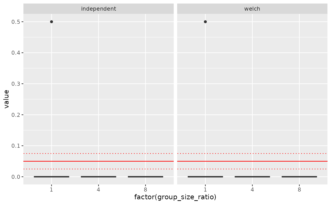
ggplot(dd, aes(factor(group_size_ratio), value)) + geom_boxplot() +
geom_abline(intercept=0.05, slope=0, col = 'red') +
geom_abline(intercept=0.075, slope=0, col = 'red', linetype='dotted') +
geom_abline(intercept=0.025, slope=0, col = 'red', linetype='dotted') +
facet_wrap(~stats)
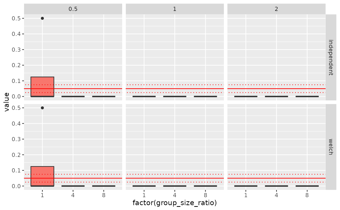
 ggplot(dd, aes(factor(group_size_ratio), value, fill = factor(standard_deviation_ratio))) +
geom_boxplot() + geom_abline(intercept=0.05, slope=0, col = 'red') +
geom_abline(intercept=0.075, slope=0, col = 'red', linetype='dotted') +
geom_abline(intercept=0.025, slope=0, col = 'red', linetype='dotted') +
facet_grid(stats~standard_deviation_ratio) +
theme(legend.position = 'none')
ggplot(dd, aes(factor(group_size_ratio), value, fill = factor(standard_deviation_ratio))) +
geom_boxplot() + geom_abline(intercept=0.05, slope=0, col = 'red') +
geom_abline(intercept=0.075, slope=0, col = 'red', linetype='dotted') +
geom_abline(intercept=0.025, slope=0, col = 'red', linetype='dotted') +
facet_grid(stats~standard_deviation_ratio) +
theme(legend.position = 'none')
 #-------------------------------------------------------------------------------
# Example with prepare() function - Loading pre-computed objects
if (FALSE) { # \dontrun{
# Step 1: Pre-generate expensive objects offline (can be parallelized)
Design <- createDesign(N = c(10, 20), rho = c(0.3, 0.7))
# Create directory for storing prepared objects
dir.create('prepared_objects', showWarnings = FALSE)
# Generate and save correlation matrices for each condition
for(i in 1:nrow(Design)) {
cond <- Design[i, ]
# Generate correlation matrix
corr_matrix <- matrix(cond$rho, nrow=cond$N, ncol=cond$N)
diag(corr_matrix) <- 1
# Create filename based on design parameters
fname <- paste0('prepared_objects/N', cond$N, '_rho', cond$rho, '.rds')
# Save to disk
saveRDS(corr_matrix, file = fname)
}
# Step 2: Use prepare() to load these objects during simulation
prepare <- function(condition, fixed_objects) {
# Create matching filename
fname <- paste0('prepared_objects/N', condition$N,
'_rho', condition$rho, '.rds')
# Load the pre-computed correlation matrix
fixed_objects$corr_matrix <- readRDS(fname)
return(fixed_objects)
}
generate <- function(condition, fixed_objects) {
# Use the loaded correlation matrix to generate multivariate data
dat <- MASS::mvrnorm(n = 50,
mu = rep(0, condition$N),
Sigma = fixed_objects$corr_matrix)
data.frame(dat)
}
analyse <- function(condition, dat, fixed_objects) {
# Calculate mean correlation in generated data
obs_corr <- cor(dat)
c(mean_corr = mean(obs_corr[lower.tri(obs_corr)]))
}
summarise <- function(condition, results, fixed_objects) {
c(mean_corr = mean(results$mean_corr))
}
# Run simulation - prepare() loads objects efficiently
results <- runSimulation(design = Design,
replications = 2,
prepare = prepare,
generate = generate,
analyse = analyse,
summarise = summarise,
verbose = FALSE)
results
# Cleanup
SimClean(dirs='prepared_objects')
} # }
#-------------------------------------------------------------------------------
# Example with prepare() function - Loading pre-computed objects
if (FALSE) { # \dontrun{
# Step 1: Pre-generate expensive objects offline (can be parallelized)
Design <- createDesign(N = c(10, 20), rho = c(0.3, 0.7))
# Create directory for storing prepared objects
dir.create('prepared_objects', showWarnings = FALSE)
# Generate and save correlation matrices for each condition
for(i in 1:nrow(Design)) {
cond <- Design[i, ]
# Generate correlation matrix
corr_matrix <- matrix(cond$rho, nrow=cond$N, ncol=cond$N)
diag(corr_matrix) <- 1
# Create filename based on design parameters
fname <- paste0('prepared_objects/N', cond$N, '_rho', cond$rho, '.rds')
# Save to disk
saveRDS(corr_matrix, file = fname)
}
# Step 2: Use prepare() to load these objects during simulation
prepare <- function(condition, fixed_objects) {
# Create matching filename
fname <- paste0('prepared_objects/N', condition$N,
'_rho', condition$rho, '.rds')
# Load the pre-computed correlation matrix
fixed_objects$corr_matrix <- readRDS(fname)
return(fixed_objects)
}
generate <- function(condition, fixed_objects) {
# Use the loaded correlation matrix to generate multivariate data
dat <- MASS::mvrnorm(n = 50,
mu = rep(0, condition$N),
Sigma = fixed_objects$corr_matrix)
data.frame(dat)
}
analyse <- function(condition, dat, fixed_objects) {
# Calculate mean correlation in generated data
obs_corr <- cor(dat)
c(mean_corr = mean(obs_corr[lower.tri(obs_corr)]))
}
summarise <- function(condition, results, fixed_objects) {
c(mean_corr = mean(results$mean_corr))
}
# Run simulation - prepare() loads objects efficiently
results <- runSimulation(design = Design,
replications = 2,
prepare = prepare,
generate = generate,
analyse = analyse,
summarise = summarise,
verbose = FALSE)
results
# Cleanup
SimClean(dirs='prepared_objects')
} # }