Full-Information Item Factor Analysis (Multidimensional Item Response Theory)

mirt fits a maximum likelihood (or maximum a posteriori) factor analysis model to any mixture of dichotomous and polytomous data under the multidimensional item response theory paradigm using either Cai's (2010) Metropolis-Hastings Robbins-Monro (MHRM) algorithm, with an EM algorithm approach outlined by Bock and Aitkin (1981) using rectangular or quasi-Monte Carlo integration grids, or with the stochastic EM (i.e., the first two stages of the MH-RM algorithm). Unidimensional and multidimensional dominance/compensatory response models or unfolding/pairwise comparison models can be specified independently via the itemtype argument.

Usage

mirt(
  data,
  model = 1,
  itemtype = NULL,
  guess = 0,
  upper = 1,
  SE = FALSE,
  covdata = NULL,
  formula = NULL,
  itemdesign = NULL,
  item.formula = NULL,
  SE.type = "Oakes",
  method = "EM",
  optimizer = NULL,
  dentype = "Gaussian",
  pars = NULL,
  constrain = NULL,
  calcNull = FALSE,
  draws = 5000,
  survey.weights = NULL,
  quadpts = NULL,
  TOL = NULL,
  gpcm_mats = list(),
  grsm.block = NULL,
  rsm.block = NULL,
  monopoly.k = 1L,
  key = NULL,
  large = FALSE,
  GenRandomPars = FALSE,
  accelerate = "Ramsay",
  verbose = TRUE,
  solnp_args = list(),
  nloptr_args = list(),
  spline_args = list(),
  control = list(),
  technical = list(),
  ...
)

Arguments

data

a matrix or data.frame that consists of numerically ordered data, organized in the form of integers, with missing data coded as NA (to convert from an ordered factor data.frame see data.matrix)

model

a string to be passed (or an object returned from) mirt.model, declaring how the IRT model is to be estimated (loadings, constraints, priors, etc). For exploratory IRT models, a single numeric value indicating the number of factors to extract is also supported. Default is 1, indicating that a unidimensional model will be fit unless otherwise specified

itemtype

type of items to be modeled, declared as either a) a single value to be recycled for each item, b) a vector for each respective item, or c) if applicable, a matrix with columns equal to the number of items and rows equal to the number of latent classes. The NULL default assumes that the items follow a graded or 2PL structure, however they may be changed to the following:

'Rasch' - Rasch/partial credit model by constraining slopes to 1 and freely estimating the variance parameters (alternatively, can be specified by applying equality constraints to the slope parameters in 'gpcm' and '2PL'; Rasch, 1960)
'1PL', '2PL', '3PL', '3PLu', and '4PL' - 1-4 parameter logistic model, where 3PL estimates the lower asymptote only while 3PLu estimates the upper asymptote only (Lord and Novick, 1968; Lord, 1980). Note that specifying '1PL' will not automatically estimate the variance of the latent trait compared to the 'Rasch' type
'5PL' - 5 parameter logistic model to estimate asymmetric logistic response curves. Currently restricted to unidimensional models
'CLL' - complementary log-log link model. Currently restricted to unidimensional models
'ULL' - unipolar log-logistic model (Lucke, 2015). Note the use of this itemtype will automatically use a log-normal distribution for the latent traits
'graded' - graded response model (Samejima, 1969)
'grsm' - graded ratings scale model in the classical IRT parameterization (restricted to unidimensional models; Muraki, 1992)
'gpcm' and 'gpcmIRT' - generalized partial credit model in the slope-intercept and classical parameterization. 'gpcmIRT' is restricted to unidimensional models. Note that optional scoring matrices for 'gpcm' are available with the gpcm_mats input (Muraki, 1992)
'rsm' - Rasch rating scale model using the 'gpcmIRT' structure (unidimensional only; Andrich, 1978)
'nominal' - nominal response model (Bock, 1972)
'ideal' - dichotomous ideal point model (Maydeu-Olivares, 2006)
'ggum' - generalized graded unfolding model (Roberts, Donoghue, & Laughlin, 2000) and its multidimensional extension
'hcm' and 'ghcm' - (generalized) hyperbolic cosine model (Andrich and Luo, 1993; Andrich, 1996) for dichotomous or ordered polytomous items (see Luo, 2001)
'alm' and 'galm' - (generalized) absolute logistic model (Luo and Andrich, 2005) for dichotomous or ordered polytomous items
'sslm' and 'gsslm' - (generalized) simple squared logistic model (Andrich, 1988) for dichotomous or ordered polytomous items (see Luo, 2001)
'paralla' and 'gparalla' - (generalized) parallellogram analysis model (Hoijtink, 1990) for dichotomous or ordered polytomous items (see Luo, 2001)
'sequential' - multidimensional sequential response model (Tutz, 1990) in slope-intercept form
'Tutz' - same as the 'sequential' itemtype, except the slopes are fixed to 1 and the latent variance terms are freely estimated (similar to the 'Rasch' itemtype input)
'PC1PL', 'PC2PL', and 'PC3PL' - 1-3 parameter partially compensatory model. Note that constraining the slopes to be equal across items will also reduce the model to Embretson's (a.k.a. Whitely's) multicomponent model (1980), while for 'PC1PL' the slopes are fixed to 1 while the latent trait variance terms are estimated
'2PLNRM', '3PLNRM', '3PLuNRM', and '4PLNRM' - 2-4 parameter nested logistic model, where 3PLNRM estimates the lower asymptote only while 3PLuNRM estimates the upper asymptote only (Suh and Bolt, 2010)
'spline' - spline response model with the bs (default) or the ns function (Winsberg, Thissen, and Wainer, 1984)
'monopoly' - monotonic polynomial model for unidimensional tests for dichotomous and polytomous response data (Falk and Cai, 2016)

Additionally, user defined item classes can also be defined using the createItem function

guess

fixed pseudo-guessing parameters. Can be entered as a single value to assign a global guessing parameter or may be entered as a numeric vector corresponding to each item

upper

fixed upper bound parameters for 4-PL model. Can be entered as a single value to assign a global guessing parameter or may be entered as a numeric vector corresponding to each item

SE

logical; estimate the standard errors by computing the parameter information matrix? See SE.type for the type of estimates available

covdata

a data.frame of data used for latent regression models

formula

an R formula (or list of formulas) indicating how the latent traits can be regressed using external covariates in covdata. If a named list of formulas is supplied (where the names correspond to the latent trait names in model) then specific regression effects can be estimated for each factor. Supplying a single formula will estimate the regression parameters for all latent traits by default

itemdesign

a data.frame with rows equal to the number of items and columns containing any item-design effects. If items should be included in the design structure (i.e., should be left in their canonical structure) then fewer rows can be used, however the rownames must be defined and matched with colnames in the data input. The item design matrix is constructed with the use of item.formula. Providing this input will fix the associated 'd' intercepts to 0, where applicable

item.formula

an R formula used to specify any intercept decomposition (e.g., the LLTM; Fischer, 1983). Note that only the right-hand side of the formula is required for compensatory models.

For non-compensatory itemtypes (e.g., 'PC1PL') the formula must include the name of the latent trait in the left hand side of the expression to indicate which of the trait specification should have their intercepts decomposed (see MLTM; Embretson, 1984)

SE.type

type of estimation method to use for calculating the parameter information matrix for computing standard errors and wald tests. Can be:

'Richardson', 'forward', or 'central' for the numerical Richardson, forward difference, and central difference evaluation of observed Hessian matrix
'crossprod' and 'Louis' for standard error computations based on the variance of the Fisher scores as well as Louis' (1982) exact computation of the observed information matrix. Note that Louis' estimates can take a long time to obtain for large sample sizes and long tests
'sandwich' for the sandwich covariance estimate based on the 'crossprod' and 'Oakes' estimates (see Chalmers, 2018, for details)
'sandwich.Louis' for the sandwich covariance estimate based on the 'crossprod' and 'Louis' estimates
'Oakes' for Oakes' (1999) method using a central difference approximation (see Chalmers, 2018, for details)
'SEM' for the supplemented EM (disables the accelerate option automatically; EM only)
'Fisher' for the expected information, 'complete' for information based on the complete-data Hessian used in EM algorithm
'MHRM' and 'FMHRM' for stochastic approximations of observed information matrix based on the Robbins-Monro filter or a fixed number of MHRM draws without the RM filter. These are the only options supported when method = 'MHRM'
'numerical' to obtain the numerical estimate from a call to optim when method = 'BL'

Note that both the 'SEM' method becomes very sensitive if the ML solution has has not been reached with sufficient precision, and may be further sensitive if the history of the EM cycles is not stable/sufficient for convergence of the respective estimates. Increasing the number of iterations (increasing NCYCLES and decreasing TOL, see below) will help to improve the accuracy, and can be run in parallel if a mirtCluster object has been defined (this will be used for Oakes' method as well). Additionally, inspecting the symmetry of the ACOV matrix for convergence issues by passing technical = list(symmetric = FALSE) can be helpful to determine if a sufficient solution has been reached

method

a character object specifying the estimation algorithm to be used. The default is 'EM', for the standard EM algorithm with fixed quadrature, 'QMCEM' for quasi-Monte Carlo EM estimation, or 'MCEM' for Monte Carlo EM estimation. The option 'MHRM' may also be passed to use the MH-RM algorithm, 'SEM' for the Stochastic EM algorithm (first two stages of the MH-RM stage using an optimizer other than a single Newton-Raphson iteration), and 'BL' for the Bock and Lieberman approach (generally not recommended for longer tests).

The 'EM' is generally effective with 1-3 factors, but methods such as the 'QMCEM', 'MCEM', 'SEM', or 'MHRM' should be used when the dimensions are 3 or more. Note that when the optimizer is stochastic the associated SE.type is automatically changed to SE.type = 'MHRM' by default to avoid the use of quadrature

optimizer

a character indicating which numerical optimizer to use. By default, the EM algorithm will use the 'BFGS' when there are no upper and lower bounds box-constraints and 'nlminb' when there are.

Other options include the Newton-Raphson ('NR'), which can be more efficient than the 'BFGS' but not as stable for more complex IRT models (such as the nominal or nested logit models) and the related 'NR1' which is also the Newton-Raphson but consists of only 1 update that has been coupled with RM Hessian (only applicable when the MH-RM algorithm is used). The MH-RM algorithm uses the 'NR1' by default, though currently the 'BFGS', 'L-BFGS-B', and 'NR' are also supported with this method (with fewer iterations by default) to emulate stochastic EM updates. As well, the 'Nelder-Mead' and 'SANN' estimators are available, but their routine use generally is not required or recommended.

Additionally, estimation subroutines from the Rsolnp and nloptr packages are available by passing the arguments 'solnp' and 'nloptr', respectively. This should be used in conjunction with the solnp_args and nloptr_args specified below. If equality constraints were specified in the model definition only the parameter with the lowest parnum in the pars = 'values' data.frame is used in the estimation vector passed to the objective function, and group hyper-parameters are omitted. Equality an inequality functions should be of the form function(p, optim_args), where optim_args is a list of internally parameters that largely can be ignored when defining constraints (though use of browser() here may be helpful)

dentype

type of density form to use for the latent trait parameters. Current options include

'Gaussian' (default) assumes a multivariate Gaussian distribution with an associated mean vector and variance-covariance matrix
'empiricalhist' or 'EH' estimates latent distribution using an empirical histogram described by Bock and Aitkin (1981). Only applicable for unidimensional models estimated with the EM algorithm. For this option, the number of cycles, TOL, and quadpts are adjusted accommodate for less precision during estimation (namely: TOL = 3e-5, NCYCLES = 2000, quadpts = 121)
'empiricalhist_Woods' or 'EHW' estimates latent distribution using an empirical histogram described by Bock and Aitkin (1981), with the same specifications as in dentype = 'empiricalhist', but with the extrapolation-interpolation method described by Woods (2007). NOTE: to improve stability in the presence of extreme response styles (i.e., all highest or lowest in each item) the technical option zeroExtreme = TRUE may be required to down-weight the contribution of these problematic patterns
'Davidian-#' estimates semi-parametric Davidian curves described by Woods and Lin (2009), where the # placeholder represents the number of Davidian parameters to estimate (e.g., 'Davidian-6' will estimate 6 smoothing parameters). By default, the number of quadpts is increased to 121, and this method is only applicable for unidimensional models estimated with the EM algorithm

Note that when itemtype = 'ULL' then a log-normal(0,1) density is used to support the unipolar scaling

pars

a data.frame with the structure of how the starting values, parameter numbers, estimation logical values, etc, are defined. The user may observe how the model defines the values by using pars = 'values', and this object can in turn be modified and input back into the estimation with pars = mymodifiedpars

constrain

a list of user declared equality constraints. To see how to define the parameters correctly use pars = 'values' initially to see how the parameters are labeled. To constrain parameters to be equal create a list with separate concatenated vectors signifying which parameters to constrain. For example, to set parameters 1 and 5 equal, and also set parameters 2, 6, and 10 equal use constrain = list(c(1,5), c(2,6,10)). Constraints can also be specified using the mirt.model syntax (recommended)

calcNull

logical; calculate the Null model for additional fit statistics (e.g., TLI)? Only applicable if the data contains no NA's and the data is not overly sparse

draws

the number of Monte Carlo draws to estimate the log-likelihood for the MH-RM algorithm. Default is 5000

survey.weights

a optional numeric vector of survey weights to apply for each case in the data (EM estimation only). If not specified, all cases are weighted equally (the standard IRT approach). The sum of the survey.weights must equal the total sample size for proper weighting to be applied

quadpts

number of quadrature points per dimension (must be larger than 2). By default the number of quadrature uses the following scheme: switch(as.character(nfact), '1'=61, '2'=31, '3'=15, '4'=9, '5'=7, 3). However, if the method input is set to 'QMCEM' and this argument is left blank then the default number of quasi-Monte Carlo integration nodes will be set to 5000 in total

TOL

convergence threshold for EM or MH-RM; defaults are .0001 and .001. If SE.type = 'SEM' and this value is not specified, the default is set to 1e-5. To evaluate the model using only the starting values pass TOL = NaN, and to evaluate the starting values without the log-likelihood pass TOL = NA

gpcm_mats

a list of matrices specifying how the scoring coefficients in the (generalized) partial credit model should be constructed. If omitted, the standard gpcm format will be used (i.e., seq(0, k, by = 1) for each trait). This input should be used if traits should be scored different for each category (e.g., matrix(c(0:3, 1,0,0,0), 4, 2) for a two-dimensional model where the first trait is scored like a gpcm, but the second trait is only positively indicated when the first category is selected). Can be used when itemtypes are 'gpcm' or 'Rasch', but only when the respective element in gpcm_mats is not NULL

grsm.block

an optional numeric vector indicating where the blocking should occur when using the grsm, NA represents items that do not belong to the grsm block (other items that may be estimated in the test data). For example, to specify two blocks of 3 with a 2PL item for the last item: grsm.block = c(rep(1,3), rep(2,3), NA). If NULL the all items are assumed to be within the same group and therefore have the same number of item categories

rsm.block

same as grsm.block, but for 'rsm' blocks

monopoly.k

a vector of values (or a single value to repeated for each item) which indicate the degree of the monotone polynomial fitted, where the monotone polynomial corresponds to monopoly.k * 2 + 1 (e.g., monopoly.k = 2 fits a 5th degree polynomial). Default is monopoly.k = 1, which fits a 3rd degree polynomial

key

a numeric vector of the response scoring key. Required when using nested logit item types, and must be the same length as the number of items used. Items that are not nested logit will ignore this vector, so use NA in item locations that are not applicable

large

a logical indicating whether unique response patterns should be obtained prior to performing the estimation so as to avoid repeating computations on identical patterns. The default TRUE provides the correct degrees of freedom for the model since all unique patterns are tallied (typically only affects goodness of fit statistics such as G2, but also will influence nested model comparison methods such as anova(mod1, mod2)), while FALSE will use the number of rows in data as a placeholder for the total degrees of freedom. As such, model objects should only be compared if all flags were set to TRUE or all were set to FALSE

Alternatively, if the collapse table of frequencies is desired for the purpose of saving computations (i.e., only computing the collapsed frequencies for the data onte-time) then a character vector can be passed with the arguement large = 'return' to return a list of all the desired table information used by mirt. This list object can then be reused by passing it back into the large argument to avoid re-tallying the data again (again, useful when the dataset are very large and computing the tabulated data is computationally burdensome). This strategy is shown below:

Compute organized data: e.g., internaldat <- mirt(Science, 1, large = 'return')
Pass the organized data to all estimation functions: e.g., mod <- mirt(Science, 1, large = internaldat)

GenRandomPars

logical; generate random starting values prior to optimization instead of using the fixed internal starting values?

accelerate

a character vector indicating the type of acceleration to use. Default is 'Ramsay', but may also be 'squarem' for the SQUAREM procedure (specifically, the gSqS3 approach) described in Varadhan and Roldand (2008). To disable the acceleration, pass 'none'

verbose

logical; print observed- (EM) or complete-data (MHRM) log-likelihood after each iteration cycle? Default is TRUE

solnp_args

a list of arguments to be passed to the solnp::solnp() function for equality constraints, inequality constraints, etc

nloptr_args

a list of arguments to be passed to the nloptr::nloptr() function for equality constraints, inequality constraints, etc

spline_args

a named list of lists containing information to be passed to the bs (default) and ns for each spline itemtype. Each element must refer to the name of the itemtype with the spline, while the internal list names refer to the arguments which are passed. For example, if item 2 were called 'read2', and item 5 were called 'read5', both of which were of itemtype 'spline' but item 5 should use the ns form, then a modified list for each input might be of the form:

spline_args = list(read2 = list(degree = 4), read5 = list(fun = 'ns', knots = c(-2, 2)))

This code input changes the bs() splines function to have a degree = 4 input, while the second element changes to the ns() function with knots set a c(-2, 2)

control

a list passed to the respective optimizers (i.e., optim(), nlminb(), etc). Additional arguments have been included for the 'NR' optimizer: 'tol' for the convergence tolerance in the M-step (default is TOL/1000), while the default number of iterations for the Newton-Raphson optimizer is 50 (modified with the 'maxit' control input)

technical

a list containing lower level technical parameters for estimation. May be:

NCYCLES: maximum number of EM or MH-RM cycles; defaults are 500 and 2000
MAXQUAD: maximum number of quadratures, which you can increase if you have more than 4GB or RAM on your PC; default 20000
theta_lim: range of integration grid for each dimension; default is c(-6, 6). Note that when itemtype = 'ULL' a log-normal distribution is used and the range is change to c(.01, and 6^2), where the second term is the square of the theta_lim input instead
set.seed: seed number used during estimation. Default is 12345
SEtol: standard error tolerance criteria for the S-EM and MHRM computation of the information matrix. Default is 1e-3
symmetric: logical; force S-EM/Oakes information matrix estimates to be symmetric? Default is TRUE so that computation of standard errors are more stable. Setting this to FALSE can help to detect solutions that have not reached the ML estimate
SEM_window: ratio of values used to define the S-EM window based on the observed likelihood differences across EM iterations. The default is c(0, 1 - SEtol), which provides nearly the very full S-EM window (i.e., nearly all EM cycles used). To use the a smaller SEM window change the window to to something like c(.9, .999) to start at a point farther into the EM history
warn: logical; include warning messages during estimation? Default is TRUE
message: logical; include general messages during estimation? Default is TRUE
customK: a numeric vector used to explicitly declare the number of response categories for each item. This should only be used when constructing mirt model for reasons other than parameter estimation (such as to obtain factor scores), and requires that the input data all have 0 as the lowest category. The format is the same as the extract.mirt(mod, 'K') slot in all converged models
customPriorFun: a custom function used to determine the normalized density for integration in the EM algorithm. Must be of the form function(Theta, Etable){...}, and return a numeric vector with the same length as number of rows in Theta. The Etable input contains the aggregated table generated from the current E-step computations. For proper integration, the returned vector should sum to 1 (i.e., normalized). Note that if using the Etable it will be NULL on the first call, therefore the prior will have to deal with this issue accordingly
zeroExtreme: logical; assign extreme response patterns a survey.weight of 0 (formally equivalent to removing these data vectors during estimation)? When dentype = 'EHW', where Woods' extrapolation is utilized, this option may be required if the extrapolation causes expected densities to tend towards positive or negative infinity. The default is FALSE
customTheta: a custom Theta grid, in matrix form, used for integration. If not defined, the grid is determined internally based on the number of quadpts
nconstrain: same specification as the constrain list argument, however imposes a negative equality constraint instead (e.g., $a12 = -a21$, which is specified as nconstrain = list(c(12, 21))). Note that each specification in the list must be of length 2, where the second element is taken to be -1 times the first element
delta: the deviation term used in numerical estimates when computing the ACOV matrix with the 'forward' or 'central' numerical approaches, as well as Oakes' method with the Richardson extrapolation. Default is 1e-5
parallel: logical; use the parallel cluster defined by mirtCluster? Default is TRUE
storeEMhistory: logical; store the iteration history when using the EM algorithm? Default is FALSE. When TRUE, use extract.mirt to extract
internal_constraints: logical; include the internal constraints when using certain IRT models (e.g., 'grsm' itemtype). Disable this if you want to use special optimizers such as the solnp. Default is TRUE
gain: a vector of two values specifying the numerator and exponent values for the RM gain function $(val1 / cycle)^val2$. Default is c(0.10, 0.75)
BURNIN: number of burn in cycles (stage 1) in MH-RM; default is 150
SEMCYCLES: number of SEM cycles (stage 2) in MH-RM; default is 100
MHDRAWS: number of Metropolis-Hasting draws to use in the MH-RM at each iteration; default is 5
MHcand: a vector of values used to tune the MH sampler. Larger values will cause the acceptance ratio to decrease. One value is required for each group in unconditional item factor analysis (mixedmirt() requires additional values for random effect). If null, these values are determined internally, attempting to tune the acceptance of the draws to be between .1 and .4
MHRM_SE_draws: number of fixed draws to use when SE=TRUE and SE.type = 'FMHRM' and the maximum number of draws when SE.type = 'MHRM'. Default is 2000
MCEM_draws: a function used to determine the number of quadrature points to draw for the 'MCEM' method. Must include one argument which indicates the iteration number of the EM cycle. Default is function(cycles) 500 + (cycles - 1)*2, which starts the number of draws at 500 and increases by 2 after each full EM iteration
info_if_converged: logical; compute the information matrix when using the MH-RM algorithm only if the model converged within a suitable number of iterations? Default is TRUE
logLik_if_converged: logical; compute the observed log-likelihood when using the MH-RM algorithm only if the model converged within a suitable number of iterations? Default is TRUE
keep_vcov_PD: logical; attempt to keep the variance-covariance matrix of the latent traits positive definite during estimation in the EM algorithm? This generally improves the convergence properties when the traits are highly correlated. Default is TRUE

...

additional arguments to be passed

Value

function returns an object of class SingleGroupClass (SingleGroupClass-class)

Details

Models containing 'explanatory' person or item level predictors can only be included by using the mixedmirt function, though latent regression models can be fit using the formula input in this function. Tests that form a two-tier or bi-factor structure should be estimated with the bfactor function, which uses a dimension reduction EM algorithm for modeling item parcels. Multiple group analyses (useful for DIF and DTF testing) are also available using the multipleGroup function.

Confirmatory and Exploratory IRT

Specification of the confirmatory item factor analysis model follows many of the rules in the structural equation modeling framework for confirmatory factor analysis. The variances of the latent factors are automatically fixed to 1 to help facilitate model identification. All parameters may be fixed to constant values or set equal to other parameters using the appropriate declarations. Confirmatory models may also contain 'explanatory' person or item level predictors, though including predictors is currently limited to the mixedmirt function.

When specifying a single number greater than 1 as the model input to mirt an exploratory IRT model will be estimated. Rotation and target matrix options are available if they are passed to generic functions such as summary-method and fscores. Factor means and variances are fixed to ensure proper identification.

If the model is an exploratory item factor analysis estimation will begin by computing a matrix of quasi-polychoric correlations. A factor analysis with nfact is then extracted and item parameters are estimated by $a_{ij} = f_{ij}/u_j$, where $f_{ij}$ is the factor loading for the jth item on the ith factor, and $u_j$ is the square root of the factor uniqueness, $\sqrt{1 - h_j^2}$. The initial intercept parameters are determined by calculating the inverse normal of the item facility (i.e., item easiness), $q_j$, to obtain $d_j = q_j / u_j$. A similar implementation is also used for obtaining initial values for polytomous items.

A note on upper and lower bound parameters

Internally the $g$ and $u$ parameters are transformed using a logit transformation ($log(x/(1-x))$), and can be reversed by using $1 / (1 + exp(-x))$ following convergence. This also applies when computing confidence intervals for these parameters, and is done so automatically if coef(mod, rawug = FALSE).

As such, when applying prior distributions to these parameters it is recommended to use a prior that ranges from negative infinity to positive infinity, such as the normally distributed prior via the 'norm' input (see mirt.model).

Convergence for quadrature methods

Unrestricted full-information factor analysis is known to have problems with convergence, and some items may need to be constrained or removed entirely to allow for an acceptable solution. As a general rule dichotomous items with means greater than .95, or items that are only .05 greater than the guessing parameter, should be considered for removal from the analysis or treated with prior parameter distributions. The same type of reasoning is applicable when including upper bound parameters as well. For polytomous items, if categories are rarely endorsed then this will cause similar issues. Also, increasing the number of quadrature points per dimension, or using the quasi-Monte Carlo integration method, may help to stabilize the estimation process in higher dimensions. Finally, solutions that are not well defined also will have difficulty converging, and can indicate that the model has been misspecified (e.g., extracting too many dimensions).

Convergence for MH-RM method

For the MH-RM algorithm, when the number of iterations grows very high (e.g., greater than 1500) or when Max Change = .2500 values are repeatedly printed to the console too often (indicating that the parameters were being constrained since they are naturally moving in steps greater than 0.25) then the model may either be ill defined or have a very flat likelihood surface, and genuine maximum-likelihood parameter estimates may be difficult to find. Standard errors are computed following the model convergence by passing SE = TRUE, to perform an addition MH-RM stage but treating the maximum-likelihood estimates as fixed points.

Additional helper functions

Additional functions are available in the package which can be useful pre- and post-estimation. These are:

mirt.model: Define the IRT model specification use special syntax. Useful for defining between and within group parameter constraints, prior parameter distributions, and specifying the slope coefficients for each factor
coef-method: Extract raw coefficients from the model, along with their standard errors and confidence intervals
summary-method: Extract standardized loadings from model. Accepts a rotate argument for exploratory item response model
anova-method: Compare nested models using likelihood ratio statistics as well as information criteria such as the AIC and BIC
residuals-method: Compute pairwise residuals between each item using methods such as the LD statistic (Chen & Thissen, 1997), as well as response pattern residuals
plot-method: Plot various types of test level plots including the test score and information functions and more
itemplot: Plot various types of item level plots, including the score, standard error, and information functions, and more
createItem: Create a customized itemtype that does not currently exist in the package
imputeMissing: Impute missing data given some computed Theta matrix
fscores: Find predicted scores for the latent traits using estimation methods such as EAP, MAP, ML, WLE, and EAPsum
wald: Compute Wald statistics follow the convergence of a model with a suitable information matrix
M2: Limited information goodness of fit test statistic based to determine how well the model fits the data
itemfit and personfit: Goodness of fit statistics at the item and person levels, such as the S-X2, infit, outfit, and more
boot.mirt: Compute estimated parameter confidence intervals via the bootstrap methods
mirtCluster: Define a cluster for the package functions to use for capitalizing on multi-core architecture to utilize available CPUs when possible. Will help to decrease estimation times for tasks that can be run in parallel

IRT Models

The parameter labels use the follow convention, here using two factors and $K$ as the total number of categories (using $k$ for specific category instances).

Rasch

Only one intercept estimated, and the latent variance of $\theta$ is freely estimated. If the data have more than two categories then a partial credit model is used instead (see 'gpcm' below). $$P(x = 1|\theta, d) = \frac{1}{1 + exp(-(\theta + d))}$$

1-4PL

Depending on the model $u$ may be equal to 1 (e.g., 3PL), $g$ may be equal to 0 (e.g., 2PL), or the as may be fixed to 1 (e.g., 1PL). $$P(x = 1|\theta, \psi) = g + \frac{(u - g)}{ 1 + exp(-(a_1 * \theta_1 + a_2 * \theta_2 + d))}$$

5PL

Currently restricted to unidimensional models $$P(x = 1|\theta, \psi) = g + \frac{(u - g)}{ 1 + exp(-(a_1 * \theta_1 + d))^S}$$ where $S$ allows for asymmetry in the response function and is transformation constrained to be greater than 0 (i.e., log(S) is estimated rather than S)

CLL

Complementary log-log model (see Shim, Bonifay, and Wiedermann, 2022) $$P(x = 1|\theta, b) = 1 - exp(-exp(\theta - b))$$ Currently restricted to unidimensional dichotomous data.

graded

ULL

The unipolar log-logistic model (ULL; Lucke, 2015) is defined the same as the graded response model, however $$P(x \le k | \theta, \psi) = \frac{\lambda_k\theta^\eta}{1 + \lambda_k\theta^\eta}$$. Internally the $\lambda$ parameters are exponentiated to keep them positive, and should therefore the reported estimates should be interpreted in log units

grsm

A more constrained version of the graded model where graded spacing is equal across item blocks and only adjusted by a single 'difficulty' parameter (c) while the latent variance of $\theta$ is freely estimated (see Muraki, 1990 for this exact form). This is restricted to unidimensional models only.

gpcm/nominal

For the gpcm the $d$ values are treated as fixed and ordered values from $0:(K-1)$ (in the nominal model $d_0$ is also set to 0). Additionally, for identification in the nominal model $ak_0 = 0$, $ak_{(K-1)} = (K - 1)$. $$P(x = k | \theta, \psi) = \frac{exp(ak_{k-1} * (a_1 * \theta_1 + a_2 * \theta_2) + d_{k-1})} {\sum_{k=1}^K exp(ak_{k-1} * (a_1 * \theta_1 + a_2 * \theta_2) + d_{k-1})}$$

For the partial credit model (when itemtype = 'Rasch'; unidimensional only) the above model is further constrained so that $ak = (0,1,\ldots, K-1)$, $a_1 = 1$, and the latent variance of $\theta_1$ is freely estimated. Alternatively, the partial credit model can be obtained by containing all the slope parameters in the gpcms to be equal. More specific scoring function may be included by passing a suitable list or matrices to the gpcm_mats input argument.

In the nominal model this parametrization helps to identify the empirical ordering of the categories by inspecting the $ak$ values. Larger values indicate that the item category is more positively related to the latent trait(s) being measured. For instance, if an item was truly ordinal (such as a Likert scale), and had 4 response categories, we would expect to see $ak_0 < ak_1 < ak_2 < ak_3$ following estimation. If on the other hand $ak_0 > ak_1$ then it would appear that the second category is less related to to the trait than the first, and therefore the second category should be understood as the 'lowest score'.

NOTE: The nominal model can become numerical unstable if poor choices for the high and low values are chosen, resulting in ak values greater than abs(10) or more. It is recommended to choose high and low anchors that cause the estimated parameters to fall between 0 and $K - 1$ either by theoretical means or by re-estimating the model with better values following convergence.

gpcmIRT and rsm

The gpcmIRT model is the classical generalized partial credit model for unidimensional response data. It will obtain the same fit as the gpcm presented above, however the parameterization allows for the Rasch/generalized rating scale model as a special case.

E.g., for a K = 4 category response model,

$$P(x = 0 | \theta, \psi) = exp(0) / G$$ $$P(x = 1 | \theta, \psi) = exp(a(\theta - b1) + c) / G$$ $$P(x = 2 | \theta, \psi) = exp(a(2\theta - b1 - b2) + 2c) / G$$ $$P(x = 3 | \theta, \psi) = exp(a(3\theta - b1 - b2 - b3) + 3c) / G$$ where $$G = exp(0) + exp(a(\theta - b1) + c) + exp(a(2\theta - b1 - b2) + 2c) + exp(a(3\theta - b1 - b2 - b3) + 3c)$$ Here $a$ is the slope parameter, the $b$ parameters are the threshold values for each adjacent category, and $c$ is the so-called difficulty parameter when a rating scale model is fitted (otherwise, $c = 0$ and it drops out of the computations).

The gpcmIRT can be constrained to the partial credit IRT model by either constraining all the slopes to be equal, or setting the slopes to 1 and freeing the latent variance parameter.

Finally, the rsm is a more constrained version of the (generalized) partial credit model where the spacing is equal across item blocks and only adjusted by a single 'difficulty' parameter (c). Note that this is analogous to the relationship between the graded model and the grsm (with an additional constraint regarding the fixed discrimination parameters).

sequential/Tutz

The multidimensional sequential response model has the form $$P(x = k | \theta, \psi) = \prod (1 - F(a_1 \theta_1 + a_2 \theta_2 + d_{sk})) F(a_1 \theta_1 + a_2 \theta_2 + d_{jk})$$ where $F(\cdot)$ is the cumulative logistic function. The Tutz variant of this model (Tutz, 1990) (via itemtype = 'Tutz') assumes that the slope terms are all equal to 1 and the latent variance terms are estimated (i.e., is a Rasch variant).

ideal

The ideal point model has the form, with the upper bound constraint on $d$ set to 0: $$P(x = 1 | \theta, \psi) = exp(-0.5 * (a_1 * \theta_1 + a_2 * \theta_2 + d)^2)$$

partcomp

Partially compensatory models consist of the product of 2PL probability curves. $$P(x = 1 | \theta, \psi) = g + (1 - g) (\frac{1}{1 + exp(-(a_1 * \theta_1 + d_1))}^c_1 * \frac{1}{1 + exp(-(a_2 * \theta_2 + d_2))}^c_2)$$

where $c_1$ and $c_2$ are binary indicator variables reflecting whether the item should include the select compensatory component (1) or not (0). Note that constraining the slopes to be equal across items will reduce the model to Embretson's (Whitely's) multicomponent model (1980).

2-4PLNRM

Nested logistic curves for modeling distractor items. Requires a scoring key. The model is broken into two components for the probability of endorsement. For successful endorsement the probability trace is the 1-4PL model, while for unsuccessful endorsement: $$P(x = 0 | \theta, \psi) = (1 - P_{1-4PL}(x = 1 | \theta, \psi)) * P_{nominal}(x = k | \theta, \psi)$$ which is the product of the complement of the dichotomous trace line with the nominal response model. In the nominal model, the slope parameters defined above are constrained to be 1's, while the last value of the $ak$ is freely estimated.

ggum

The (multidimensional) generalized graded unfolding model is a class of ideal point models useful for ordinal response data. The form is $$P(z=k|\theta,\psi)=\frac{exp\left[\left(z\sqrt{\sum_{d=1}^{D} a_{id}^{2}(\theta_{jd}-b_{id})^{2}}\right)+\sum_{k=0}^{z}\psi_{ik}\right]+ exp\left[\left((M-z)\sqrt{\sum_{d=1}^{D}a_{id}^{2}(\theta_{jd}-b_{id})^{2}}\right)+ \sum_{k=0}^{z}\psi_{ik}\right]}{\sum_{w=0}^{C}\left(exp\left[\left(w \sqrt{\sum_{d=1}^{D}a_{id}^{2}(\theta_{jd}-b_{id})^{2}}\right)+ \sum_{k=0}^{z}\psi_{ik}\right]+exp\left[\left((M-w) \sqrt{\sum_{d=1}^{D}a_{id}^{2}(\theta_{jd}-b_{id})^{2}}\right)+ \sum_{k=0}^{z}\psi_{ik}\right]\right)}$$ where $\theta_{jd}$ is the location of the $j$th individual on the $d$th dimension, $b_{id}$ is the difficulty location of the $i$th item on the $d$th dimension, $a_{id}$ is the discrimination of the $j$th individual on the $d$th dimension (where the discrimination values are constrained to be positive), $\psi_{ik}$ is the $k$th subjective response category threshold for the $i$th item, assumed to be symmetric about the item and constant across dimensions, where $\psi_{ik} = \sum_{d=1}^D a_{id} t_{ik}$ $z = 1,2,\ldots, C$ (where $C$ is the number of categories minus 1), and $M = 2C + 1$.

(g)hcm, (g)alm, (g)sslm, and (g)paralla

Following Luo (2001), this family of response models can be characterized under the same ordinal response functioning structure, differing only in their linking functions ($\psi(x)$). For example, for a two-dimensional model the equation used is $$p_k = \frac{\psi (\rho_k)}{\psi (\rho_k) + \psi (a_1 \theta_1 + a_2 \theta_2 + d)} $$ which is expressed in slope-intercept form to accommodate multidimensionality. The "generalized" versions of this family estimate the slope and rho parameters, which allow each item to differ in the steepness of the unfolding model functions; otherwise, slopes are fixed to the value of 1, though the rho parameters must be set to 0 manually. For ordered polytomous items the response function follows the Guttman-scaling logic $$P_1 = q_1\cdot q_2 \cdot q_3 \cdots q_k$$ $$P_2 = p_1\cdot q_2 \cdot q_3 \cdots q_k$$ $$P_3 = p_1\cdot p_2 \cdot q_3 \cdots q_k$$ $$\cdots$$ $$P_K = p_1\cdot p_2 \cdot p_3 \cdots p_k$$ Note that for estimation purposes the rho parameters are expressed in log units so that they remain positive during estimation. Hence, the parameterization used herein is $$p_k = \frac{\psi (exp(\rho^*_k))}{\psi (exp(\rho^*_k))) + \psi (a_1 \theta_1 + a_2 \theta_2 + d)} $$ where $\rho^*_k$ is in natural log units. Currently supported models in this family are the:

(generalized) hyperbolic cosine model ($\psi (x) = cosh(x)$),
(generalized) absolute logistic model ($\psi (x) = exp(|x|)$),
(generalized) simple squared logistic model ($\psi (x) = exp(x^2)$), and
(generalized) parallellogram analysis model ($\psi (x) = x^2$), respectively.

all of which are available for dichotomous and ordered polytomous response option items.

spline

Spline response models attempt to model the response curves uses non-linear and potentially non-monotonic patterns. The form is $$P(x = 1|\theta, \eta) = \frac{1}{1 + exp(-(\eta_1 * X_1 + \eta_2 * X_2 + \cdots + \eta_n * X_n))}$$ where the $X_n$ are from the spline design matrix $X$ organized from the grid of $\theta$ values. B-splines with a natural or polynomial basis are supported, and the intercept input is set to TRUE by default.

monopoly

Monotone polynomial model for polytomous response data of the form $$P(x = k | \theta, \psi) = \frac{exp(\sum_1^k (m^*(\psi) + \xi_{c-1})} {\sum_1^C exp(\sum_1^K (m^*(\psi) + \xi_{c-1}))}$$ where $m^*(\psi)$ is the monotone polynomial function without the intercept.

HTML help files, exercises, and examples

To access examples, vignettes, and exercise files that have been generated with knitr please visit https://github.com/philchalmers/mirt/wiki.

References

Andrich, D. (1978). A rating scale formulation for ordered response categories. Psychometrika, 43, 561-573.

Andrich, D. (1996). Hyperbolic cosine latent trait models for unfolding direct-responses and pairwise preferences. Applied Psychological Measurement, 20, 269-290.

Andrich, D., and Luo, G. (1993). A hyperbolic cosine latent trait model for unfolding dichotomous single- stimulus responses. Applied Psychological Measurement, 17, 253-276.

Andrich, D. (1988). The application of an unfolding model of the PIRT type to the measurement of attitude. Applied Psychological Measurement, 12, 33-51.

Bock, R. D., & Aitkin, M. (1981). Marginal maximum likelihood estimation of item parameters: Application of an EM algorithm. Psychometrika, 46(4), 443-459.

Bock, R. D., Gibbons, R., & Muraki, E. (1988). Full-Information Item Factor Analysis. Applied Psychological Measurement, 12(3), 261-280.

Bock, R. D. & Lieberman, M. (1970). Fitting a response model for n dichotomously scored items. Psychometrika, 35, 179-197.

Cai, L. (2010a). High-Dimensional exploratory item factor analysis by a Metropolis-Hastings Robbins-Monro algorithm. Psychometrika, 75, 33-57.

Cai, L. (2010b). Metropolis-Hastings Robbins-Monro algorithm for confirmatory item factor analysis. Journal of Educational and Behavioral Statistics, 35, 307-335.

Chalmers, R., P. (2012). mirt: A Multidimensional Item Response Theory Package for the R Environment. Journal of Statistical Software, 48(6), 1-29. doi:10.18637/jss.v048.i06

Chalmers, R. P. (2015). Extended Mixed-Effects Item Response Models with the MH-RM Algorithm. Journal of Educational Measurement, 52, 200-222. doi:10.1111/jedm.12072

Chalmers, R. P. (2018). Numerical Approximation of the Observed Information Matrix with Oakes' Identity. British Journal of Mathematical and Statistical Psychology DOI: 10.1111/bmsp.12127

Chalmers, R., P. & Flora, D. (2014). Maximum-likelihood Estimation of Noncompensatory IRT Models with the MH-RM Algorithm. Applied Psychological Measurement, 38, 339-358. doi:10.1177/0146621614520958

Chen, W. H. & Thissen, D. (1997). Local dependence indices for item pairs using item response theory. Journal of Educational and Behavioral Statistics, 22, 265-289.

Embretson, S. E. (1984). A general latent trait model for response processes. Psychometrika, 49, 175-186.

Falk, C. F. & Cai, L. (2016). Maximum Marginal Likelihood Estimation of a Monotonic Polynomial Generalized Partial Credit Model with Applications to Multiple Group Analysis. Psychometrika, 81, 434-460.

Fischer, G. H. (1983). Logistic latent trait models with linear constraints. Psychometrika, 48, 3-26.

Hoijtink H. (1990). PARELLA: Measurement of latent traits by proximity items. The Netherlands: University of Groningen.

Lord, F. M. & Novick, M. R. (1968). Statistical theory of mental test scores. Addison-Wesley.

Lucke, J. F. (2015). Unipolar item response models. In S. P. Reise & D. A. Revicki (Eds.), Handbook of item response theory modeling: Applications to typical performance assessment (pp. 272-284). New York, NY: Routledge/Taylor & Francis Group.

Luo G. (2001). A class of probabilistic unfolding models for polytomous responses. Journal of Mathematical Psychology. 45(2):224-248. 10.1006/jmps.2000.1310

Luo G, and Andrich D. (2005). Information functions for the general dichotomous unfolding model. In: Alagumalai S, Curtis D.D., & Hungi N., editor. Applied Rasch Measurement: A Book of Exemplars: Dordrecht, The Netherlands: Springer.

Maydeu-Olivares, A., Hernandez, A. & McDonald, R. P. (2006). A Multidimensional Ideal Point Item Response Theory Model for Binary Data. Multivariate Behavioral Research, 41, 445-471.

Muraki, E. (1990). Fitting a polytomous item response model to Likert-type data. Applied Psychological Measurement, 14, 59-71.

Muraki, E. (1992). A generalized partial credit model: Application of an EM algorithm. Applied Psychological Measurement, 16, 159-176.

Muraki, E. & Carlson, E. B. (1995). Full-information factor analysis for polytomous item responses. Applied Psychological Measurement, 19, 73-90.

Ramsay, J. O. (1975). Solving implicit equations in psychometric data analysis. Psychometrika, 40, 337-360.

Rasch, G. (1960). Probabilistic models for some intelligence and attainment tests. Danish Institute for Educational Research.

Roberts, J. S., Donoghue, J. R., & Laughlin, J. E. (2000). A General Item Response Theory Model for Unfolding Unidimensional Polytomous Responses. Applied Psychological Measurement, 24, 3-32.

Samejima, F. (1969). Estimation of latent ability using a response pattern of graded scores. Psychometrika Monographs, 34.

Shim, H., Bonifay, W., & Wiedermann, W. (2022). Parsimonious asymmetric item response theory modeling with the complementary log-log link. Behavior Research Methods, 55, 200-219.

Suh, Y. & Bolt, D. (2010). Nested logit models for multiple-choice item response data. Psychometrika, 75, 454-473.

Sympson, J. B. (1977). A model for testing with multidimensional items. Proceedings of the 1977 Computerized Adaptive Testing Conference.

Thissen, D. (1982). Marginal maximum likelihood estimation for the one-parameter logistic model. Psychometrika, 47, 175-186.

Tutz, G. (1990). Sequential item response models with ordered response. British Journal of Mathematical and Statistical Psychology, 43, 39-55.

Varadhan, R. & Roland, C. (2008). Simple and Globally Convergent Methods for Accelerating the Convergence of Any EM Algorithm. Scandinavian Journal of Statistics, 35, 335-353.

Whitely, S. E. (1980). Multicomponent latent trait models for ability tests. Psychometrika, 45(4), 470-494.

Wood, R., Wilson, D. T., Gibbons, R. D., Schilling, S. G., Muraki, E., & Bock, R. D. (2003). TESTFACT 4 for Windows: Test Scoring, Item Statistics, and Full-information Item Factor Analysis [Computer software]. Lincolnwood, IL: Scientific Software International.

Woods, C. M., and Lin, N. (2009). Item Response Theory With Estimation of the Latent Density Using Davidian Curves. Applied Psychological Measurement,33(2), 102-117.

Author

Phil Chalmers rphilip.chalmers@gmail.com

Examples


# load LSAT section 7 data and compute 1 and 2 factor models
data <- expand.table(LSAT7)
itemstats(data)
#> $overall
#>     N mean_total.score sd_total.score ave.r  sd.r alpha SEM.alpha
#>  1000            3.707          1.199 0.143 0.052 0.453     0.886
#> 
#> $itemstats
#>           N  mean    sd total.r total.r_if_rm alpha_if_rm
#> Item.1 1000 0.828 0.378   0.530         0.246       0.396
#> Item.2 1000 0.658 0.475   0.600         0.247       0.394
#> Item.3 1000 0.772 0.420   0.611         0.313       0.345
#> Item.4 1000 0.606 0.489   0.592         0.223       0.415
#> Item.5 1000 0.843 0.364   0.461         0.175       0.438
#> 
#> $proportions
#>            0     1
#> Item.1 0.172 0.828
#> Item.2 0.342 0.658
#> Item.3 0.228 0.772
#> Item.4 0.394 0.606
#> Item.5 0.157 0.843
#> 

(mod1 <- mirt(data, 1))
#> 
#> 
#> Call:
#> mirt(data = data, model = 1)
#> 
#> Full-information item factor analysis with 1 factor(s).
#> Converged within 1e-04 tolerance after 28 EM iterations.
#> mirt version: 1.44.5 
#> M-step optimizer: BFGS 
#> EM acceleration: Ramsay 
#> Number of rectangular quadrature: 61
#> Latent density type: Gaussian 
#> 
#> Log-likelihood = -2658.805
#> Estimated parameters: 10 
#> AIC = 5337.61
#> BIC = 5386.688; SABIC = 5354.927
#> G2 (21) = 31.7, p = 0.0628
#> RMSEA = 0.023, CFI = NaN, TLI = NaN
coef(mod1)
#> $Item.1
#>        a1     d g u
#> par 0.988 1.856 0 1
#> 
#> $Item.2
#>        a1     d g u
#> par 1.081 0.808 0 1
#> 
#> $Item.3
#>        a1     d g u
#> par 1.706 1.804 0 1
#> 
#> $Item.4
#>        a1     d g u
#> par 0.765 0.486 0 1
#> 
#> $Item.5
#>        a1     d g u
#> par 0.736 1.855 0 1
#> 
#> $GroupPars
#>     MEAN_1 COV_11
#> par      0      1
#> 
summary(mod1)
#>           F1    h2
#> Item.1 0.502 0.252
#> Item.2 0.536 0.287
#> Item.3 0.708 0.501
#> Item.4 0.410 0.168
#> Item.5 0.397 0.157
#> 
#> SS loadings:  1.366 
#> Proportion Var:  0.273 
#> 
#> Factor correlations: 
#> 
#>    F1
#> F1  1
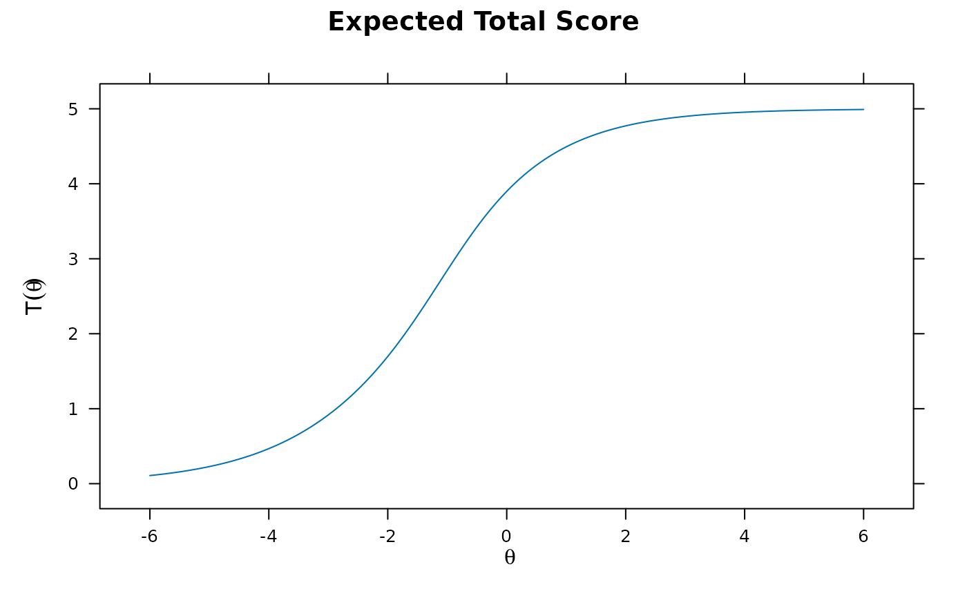
plot(mod1)

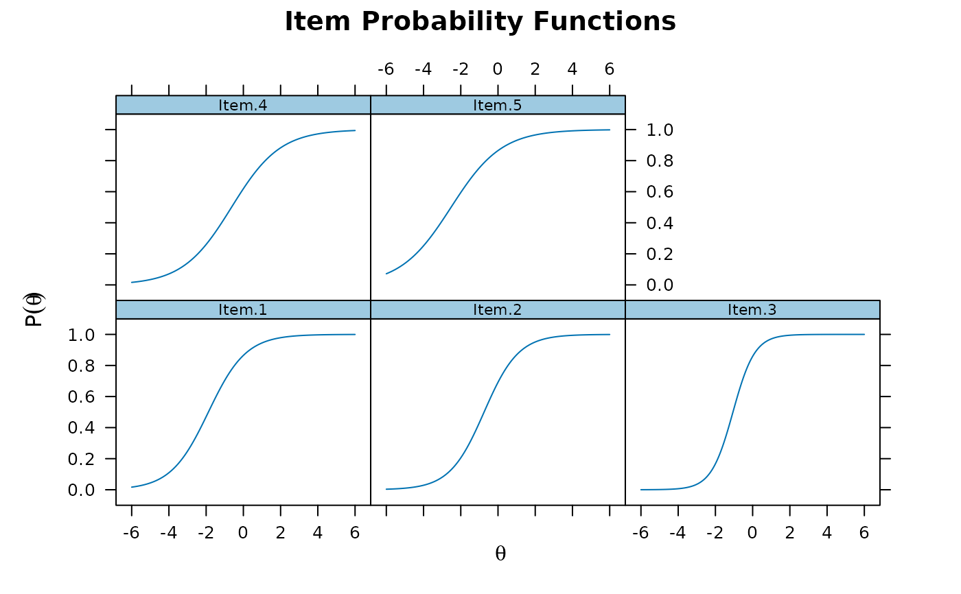
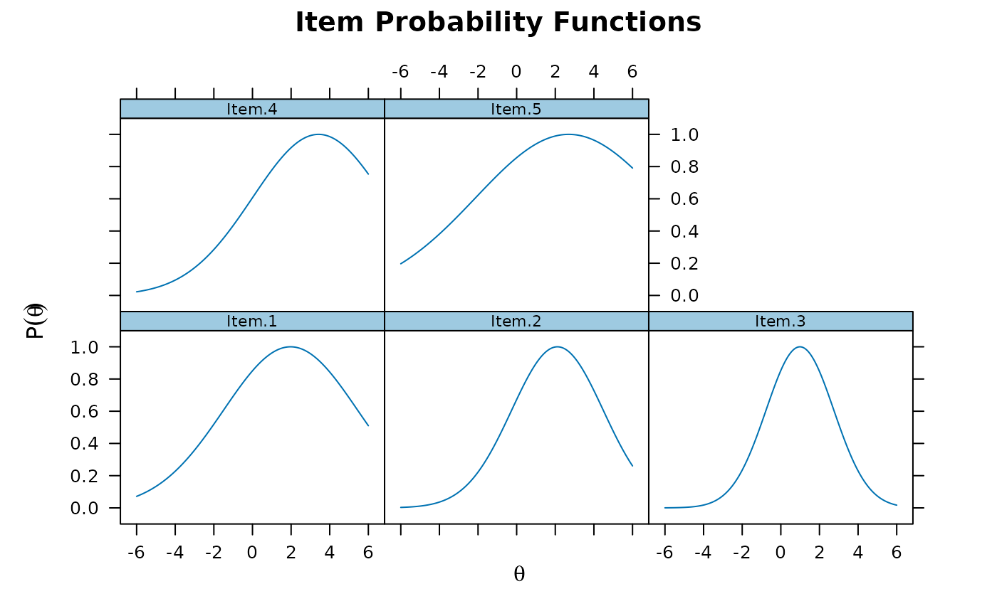
plot(mod1, type = 'trace')


# \donttest{
(mod2 <- mirt(data, 1, SE = TRUE)) #standard errors via the Oakes method
#> 
#> 
#> Calculating information matrix...
#> 
#> Call:
#> mirt(data = data, model = 1, SE = TRUE)
#> 
#> Full-information item factor analysis with 1 factor(s).
#> Converged within 1e-04 tolerance after 28 EM iterations.
#> mirt version: 1.44.5 
#> M-step optimizer: BFGS 
#> EM acceleration: Ramsay 
#> Number of rectangular quadrature: 61
#> Latent density type: Gaussian 
#> 
#> Information matrix estimated with method: Oakes
#> Second-order test: model is a possible local maximum
#> Condition number of information matrix =  30.23088
#> 
#> Log-likelihood = -2658.805
#> Estimated parameters: 10 
#> AIC = 5337.61
#> BIC = 5386.688; SABIC = 5354.927
#> G2 (21) = 31.7, p = 0.0628
#> RMSEA = 0.023, CFI = NaN, TLI = NaN
(mod2 <- mirt(data, 1, SE = TRUE, SE.type = 'SEM')) #standard errors with SEM method
#> 
#> 
#> Calculating information matrix...
#> 
#> Call:
#> mirt(data = data, model = 1, SE = TRUE, SE.type = "SEM")
#> 
#> Full-information item factor analysis with 1 factor(s).
#> Converged within 1e-05 tolerance after 74 EM iterations.
#> mirt version: 1.44.5 
#> M-step optimizer: BFGS 
#> EM acceleration: none 
#> Number of rectangular quadrature: 61
#> Latent density type: Gaussian 
#> 
#> Information matrix estimated with method: SEM
#> Second-order test: model is a possible local maximum
#> Condition number of information matrix =  30.12751
#> 
#> Log-likelihood = -2658.805
#> Estimated parameters: 10 
#> AIC = 5337.61
#> BIC = 5386.688; SABIC = 5354.927
#> G2 (21) = 31.7, p = 0.0628
#> RMSEA = 0.023, CFI = NaN, TLI = NaN
coef(mod2)
#> $Item.1
#>            a1     d  g  u
#> par     0.988 1.856  0  1
#> CI_2.5  0.639 1.599 NA NA
#> CI_97.5 1.336 2.112 NA NA
#> 
#> $Item.2
#>            a1     d  g  u
#> par     1.081 0.808  0  1
#> CI_2.5  0.755 0.629 NA NA
#> CI_97.5 1.407 0.987 NA NA
#> 
#> $Item.3
#>            a1     d  g  u
#> par     1.707 1.805  0  1
#> CI_2.5  1.086 1.395 NA NA
#> CI_97.5 2.329 2.215 NA NA
#> 
#> $Item.4
#>            a1     d  g  u
#> par     0.765 0.486  0  1
#> CI_2.5  0.500 0.339 NA NA
#> CI_97.5 1.030 0.633 NA NA
#> 
#> $Item.5
#>            a1     d  g  u
#> par     0.736 1.854  0  1
#> CI_2.5  0.437 1.630 NA NA
#> CI_97.5 1.034 2.079 NA NA
#> 
#> $GroupPars
#>         MEAN_1 COV_11
#> par          0      1
#> CI_2.5      NA     NA
#> CI_97.5     NA     NA
#> 
(mod3 <- mirt(data, 1, SE = TRUE, SE.type = 'Richardson')) #with numerical Richardson method
#> 
#> 
#> Calculating information matrix...
#> 
#> Call:
#> mirt(data = data, model = 1, SE = TRUE, SE.type = "Richardson")
#> 
#> Full-information item factor analysis with 1 factor(s).
#> Converged within 1e-04 tolerance after 28 EM iterations.
#> mirt version: 1.44.5 
#> M-step optimizer: BFGS 
#> EM acceleration: Ramsay 
#> Number of rectangular quadrature: 61
#> Latent density type: Gaussian 
#> 
#> Information matrix estimated with method: Richardson
#> Second-order test: model is a possible local maximum
#> Condition number of information matrix =  30.23102
#> 
#> Log-likelihood = -2658.805
#> Estimated parameters: 10 
#> AIC = 5337.61
#> BIC = 5386.688; SABIC = 5354.927
#> G2 (21) = 31.7, p = 0.0628
#> RMSEA = 0.023, CFI = NaN, TLI = NaN
residuals(mod1)
#> LD matrix (lower triangle) and standardized residual correlations (upper triangle)
#> 
#> Upper triangle summary:
#>    Min. 1st Qu.  Median    Mean 3rd Qu.    Max. 
#>  -0.037  -0.020  -0.007   0.001   0.024   0.051 
#> 
#>        Item.1 Item.2 Item.3 Item.4 Item.5
#> Item.1        -0.021 -0.029  0.051  0.049
#> Item.2  0.453         0.033 -0.016 -0.037
#> Item.3  0.854  1.060        -0.012 -0.002
#> Item.4  2.572  0.267  0.153         0.000
#> Item.5  2.389  1.384  0.003  0.000       
plot(mod1) #test score function

plot(mod1, type = 'trace') #trace lines

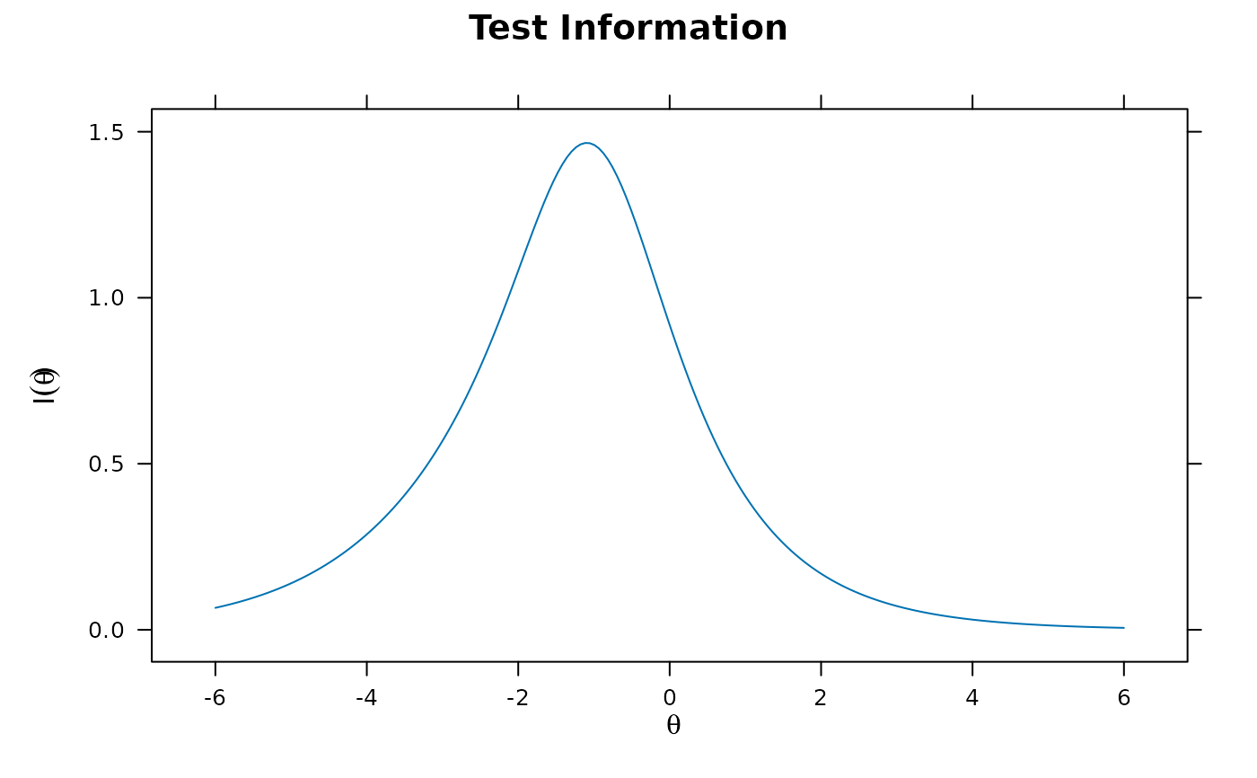
plot(mod2, type = 'info') #test information

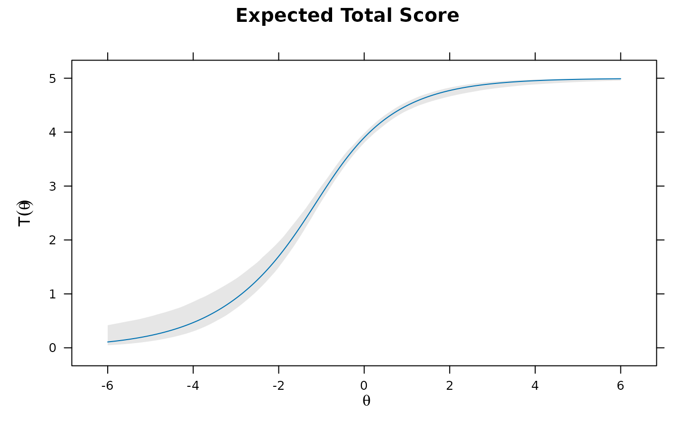
plot(mod2, MI=200) #expected total score with 95% confidence intervals


# estimated 3PL model for item 5 only
(mod1.3PL <- mirt(data, 1, itemtype = c('2PL', '2PL', '2PL', '2PL', '3PL')))
#> 
#> 
#> Call:
#> mirt(data = data, model = 1, itemtype = c("2PL", "2PL", "2PL", 
#>     "2PL", "3PL"))
#> 
#> Full-information item factor analysis with 1 factor(s).
#> Converged within 1e-04 tolerance after 43 EM iterations.
#> mirt version: 1.44.5 
#> M-step optimizer: BFGS 
#> EM acceleration: Ramsay 
#> Number of rectangular quadrature: 61
#> Latent density type: Gaussian 
#> 
#> Log-likelihood = -2658.794
#> Estimated parameters: 11 
#> AIC = 5339.587
#> BIC = 5393.573; SABIC = 5358.636
#> G2 (20) = 31.68, p = 0.0469
#> RMSEA = 0.024, CFI = NaN, TLI = NaN
coef(mod1.3PL)
#> $Item.1
#>        a1     d g u
#> par 0.987 1.855 0 1
#> 
#> $Item.2
#>        a1     d g u
#> par 1.082 0.808 0 1
#> 
#> $Item.3
#>        a1     d g u
#> par 1.706 1.805 0 1
#> 
#> $Item.4
#>        a1     d g u
#> par 0.764 0.486 0 1
#> 
#> $Item.5
#>        a1     d     g u
#> par 0.778 1.643 0.161 1
#> 
#> $GroupPars
#>     MEAN_1 COV_11
#> par      0      1
#> 

# internally g and u pars are stored as logits, so usually a good idea to include normal prior
#  to help stabilize the parameters. For a value around .182 use a mean
#  of -1.5 (since 1 / (1 + exp(-(-1.5))) == .182)
model <- 'F = 1-5
         PRIOR = (5, g, norm, -1.5, 3)'
mod1.3PL.norm <- mirt(data, model, itemtype = c('2PL', '2PL', '2PL', '2PL', '3PL'))
#> 
coef(mod1.3PL.norm)
#> $Item.1
#>        a1     d g u
#> par 0.987 1.855 0 1
#> 
#> $Item.2
#>        a1     d g u
#> par 1.083 0.808 0 1
#> 
#> $Item.3
#>        a1     d g u
#> par 1.706 1.804 0 1
#> 
#> $Item.4
#>        a1     d g u
#> par 0.764 0.486 0 1
#> 
#> $Item.5
#>        a1   d    g u
#> par 0.788 1.6 0.19 1
#> 
#> $GroupPars
#>     MEAN_1 COV_11
#> par      0      1
#> 
#limited information fit statistics
M2(mod1.3PL.norm)
#>             M2 df          p      RMSEA RMSEA_5   RMSEA_95      SRMSR       TLI
#> stats 8.800082  4 0.06629543 0.03465864       0 0.06610847 0.03207363 0.9454563
#>             CFI
#> stats 0.9781825

# unidimensional ideal point model
idealpt <- mirt(data, 1, itemtype = 'ideal')
#> 
plot(idealpt, type = 'trace', facet_items = TRUE)

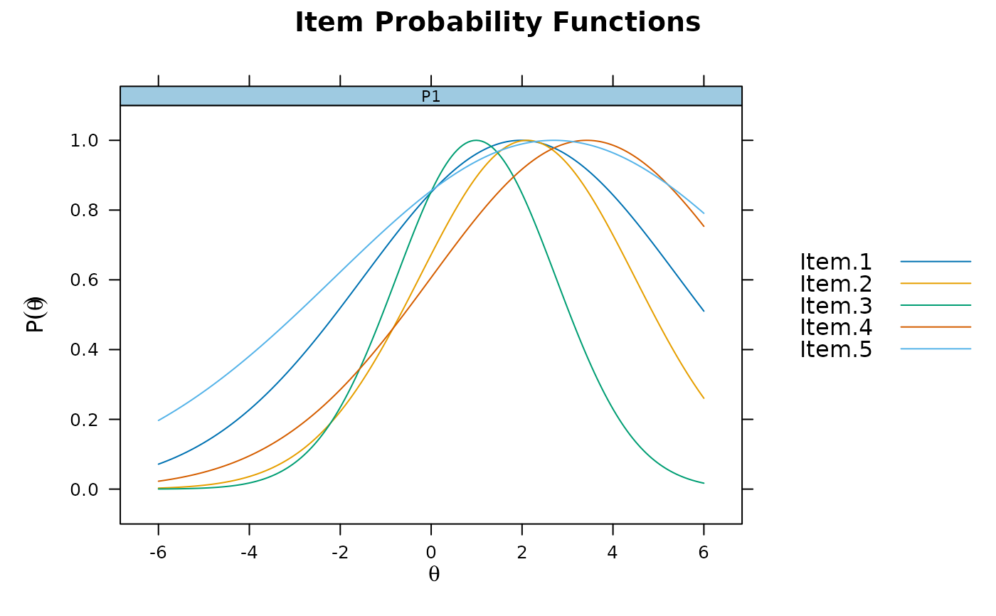
plot(idealpt, type = 'trace', facet_items = FALSE)


# two factors (exploratory)
mod2 <- mirt(data, 2)
#> 
coef(mod2)
#> $Item.1
#>         a1   a2     d g u
#> par -2.007 0.87 2.648 0 1
#> 
#> $Item.2
#>         a1     a2     d g u
#> par -0.849 -0.522 0.788 0 1
#> 
#> $Item.3
#>         a1     a2     d g u
#> par -2.153 -1.836 2.483 0 1
#> 
#> $Item.4
#>         a1     a2     d g u
#> par -0.756 -0.028 0.485 0 1
#> 
#> $Item.5
#>         a1 a2     d g u
#> par -0.757  0 1.864 0 1
#> 
#> $GroupPars
#>     MEAN_1 MEAN_2 COV_11 COV_21 COV_22
#> par      0      0      1      0      1
#> 
summary(mod2, rotate = 'oblimin') #oblimin rotation
#> 
#> Rotation:  oblimin 
#> 
#> Rotated factor loadings: 
#> 
#>             F1      F2    h2
#> Item.1  0.7944 -0.0111 0.623
#> Item.2  0.0804  0.4630 0.255
#> Item.3 -0.0129  0.8628 0.734
#> Item.4  0.2794  0.1925 0.165
#> Item.5  0.2929  0.1772 0.165
#> 
#> Rotated SS loadings:  0.802 1.027 
#> 
#> Factor correlations: 
#> 
#>       F1 F2
#> F1 1.000   
#> F2 0.463  1
residuals(mod2)
#> LD matrix (lower triangle) and standardized residual correlations (upper triangle)
#> 
#> Upper triangle summary:
#>    Min. 1st Qu.  Median    Mean 3rd Qu.    Max. 
#>  -0.018  -0.001   0.000   0.000   0.002   0.011 
#> 
#>        Item.1 Item.2 Item.3 Item.4 Item.5
#> Item.1        -0.001  0.001  0.002  0.003
#> Item.2  0.001         0.000  0.011 -0.018
#> Item.3  0.001  0.000        -0.002  0.006
#> Item.4  0.002  0.111  0.004        -0.001
#> Item.5  0.008  0.325  0.041  0.001       
plot(mod2)

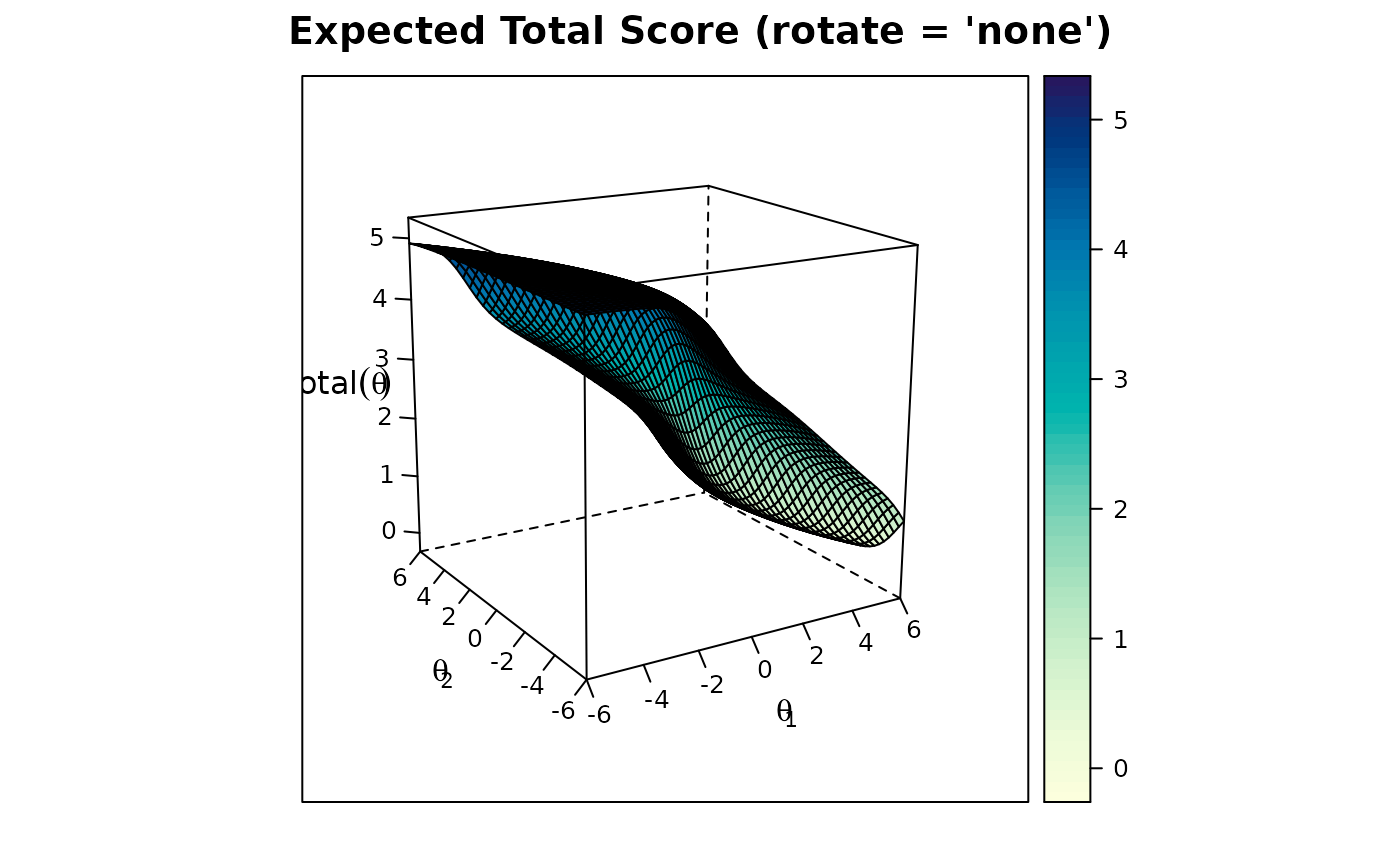plot(mod2, rotate = 'oblimin')


anova(mod1, mod2) #compare the two models
#>           AIC    SABIC       HQ      BIC    logLik     X2 df     p
#> mod1 5337.610 5354.927 5356.263 5386.688 -2658.805                
#> mod2 5335.039 5359.283 5361.153 5403.748 -2653.520 10.571  4 0.032
scoresfull <- fscores(mod2) #factor scores for each response pattern
head(scoresfull)
#>             F1        F2
#> [1,] -1.700513 -1.711766
#> [2,] -1.700513 -1.711766
#> [3,] -1.700513 -1.711766
#> [4,] -1.700513 -1.711766
#> [5,] -1.700513 -1.711766
#> [6,] -1.700513 -1.711766
scorestable <- fscores(mod2, full.scores = FALSE) #save factor score table
#> 
#> Method:  EAP
#> Rotate:  oblimin
#> 
#> Empirical Reliability:
#> 
#>     F1     F2 
#> 0.2717 0.3565 
head(scorestable)
#>      Item.1 Item.2 Item.3 Item.4 Item.5        F1         F2     SE_F1
#> [1,]      0      0      0      0      0 -1.700513 -1.7117658 0.8233498
#> [2,]      0      0      0      0      1 -1.442213 -1.5315319 0.8291596
#> [3,]      0      0      0      1      0 -1.448997 -1.5246522 0.8289670
#> [4,]      0      0      0      1      1 -1.186286 -1.3432706 0.8376135
#> [5,]      0      0      1      0      0 -1.369479 -0.7080874 0.8344669
#> [6,]      0      0      1      0      1 -1.099364 -0.5102905 0.8455289
#>          SE_F2
#> [1,] 0.7705787
#> [2,] 0.7691522
#> [3,] 0.7691142
#> [4,] 0.7711322
#> [5,] 0.7962954
#> [6,] 0.8101333

# confirmatory (as an example, model is not identified since you need 3 items per factor)
# Two ways to define a confirmatory model: with mirt.model, or with a string

# these model definitions are equivalent
cmodel <- mirt.model('
   F1 = 1,4,5
   F2 = 2,3')
cmodel2 <- 'F1 = 1,4,5
            F2 = 2,3'

cmod <- mirt(data, cmodel)
#> 
# cmod <- mirt(data, cmodel2) # same as above
coef(cmod)
#> $Item.1
#>        a1 a2     d g u
#> par 1.792  0 2.358 0 1
#> 
#> $Item.2
#>     a1    a2   d g u
#> par  0 1.427 0.9 0 1
#> 
#> $Item.3
#>     a1    a2     d g u
#> par  0 1.559 1.725 0 1
#> 
#> $Item.4
#>        a1 a2     d g u
#> par 0.743  0 0.483 0 1
#> 
#> $Item.5
#>        a1 a2     d g u
#> par 0.763  0 1.867 0 1
#> 
#> $GroupPars
#>     MEAN_1 MEAN_2 COV_11 COV_21 COV_22
#> par      0      0      1      0      1
#> 
anova(cmod, mod2)
#>           AIC    SABIC       HQ      BIC    logLik     X2 df p
#> cmod 5392.596 5409.913 5411.249 5441.674 -2686.298            
#> mod2 5335.039 5359.283 5361.153 5403.748 -2653.520 65.557  4 0
# check if identified by computing information matrix
(cmod <- mirt(data, cmodel, SE = TRUE))
#> 
#> 
#> Calculating information matrix...
#> Warning: Could not invert information matrix; model may not be (empirically) identified.
#> 
#> Call:
#> mirt(data = data, model = cmodel, SE = TRUE)
#> 
#> Full-information item factor analysis with 2 factor(s).
#> Converged within 1e-04 tolerance after 125 EM iterations.
#> mirt version: 1.44.5 
#> M-step optimizer: BFGS 
#> EM acceleration: Ramsay 
#> Number of rectangular quadrature: 31
#> Latent density type: Gaussian 
#> 
#> Information matrix estimated with method: Oakes
#> Second-order test: model is not a maximum or the information matrix is too inaccurate
#> 
#> Log-likelihood = -2686.298
#> Estimated parameters: 10 
#> AIC = 5392.596
#> BIC = 5441.674; SABIC = 5409.913
#> G2 (21) = 86.69, p = 0
#> RMSEA = 0.056, CFI = NaN, TLI = NaN

###########
# data from the 'ltm' package in numeric format
itemstats(Science)
#> $overall
#>    N mean_total.score sd_total.score ave.r  sd.r alpha SEM.alpha
#>  392           11.668          2.003 0.275 0.098 0.598      1.27
#> 
#> $itemstats
#>           N  mean    sd total.r total.r_if_rm alpha_if_rm
#> Comfort 392 3.120 0.588   0.596         0.352       0.552
#> Work    392 2.722 0.807   0.666         0.332       0.567
#> Future  392 2.990 0.757   0.748         0.488       0.437
#> Benefit 392 2.837 0.802   0.684         0.363       0.541
#> 
#> $proportions
#>             1     2     3     4
#> Comfort 0.013 0.082 0.679 0.227
#> Work    0.084 0.250 0.526 0.140
#> Future  0.036 0.184 0.536 0.245
#> Benefit 0.054 0.255 0.492 0.199
#> 

pmod1 <- mirt(Science, 1)
#> 
plot(pmod1)

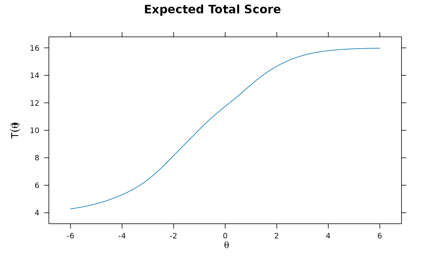plot(pmod1, type = 'trace')

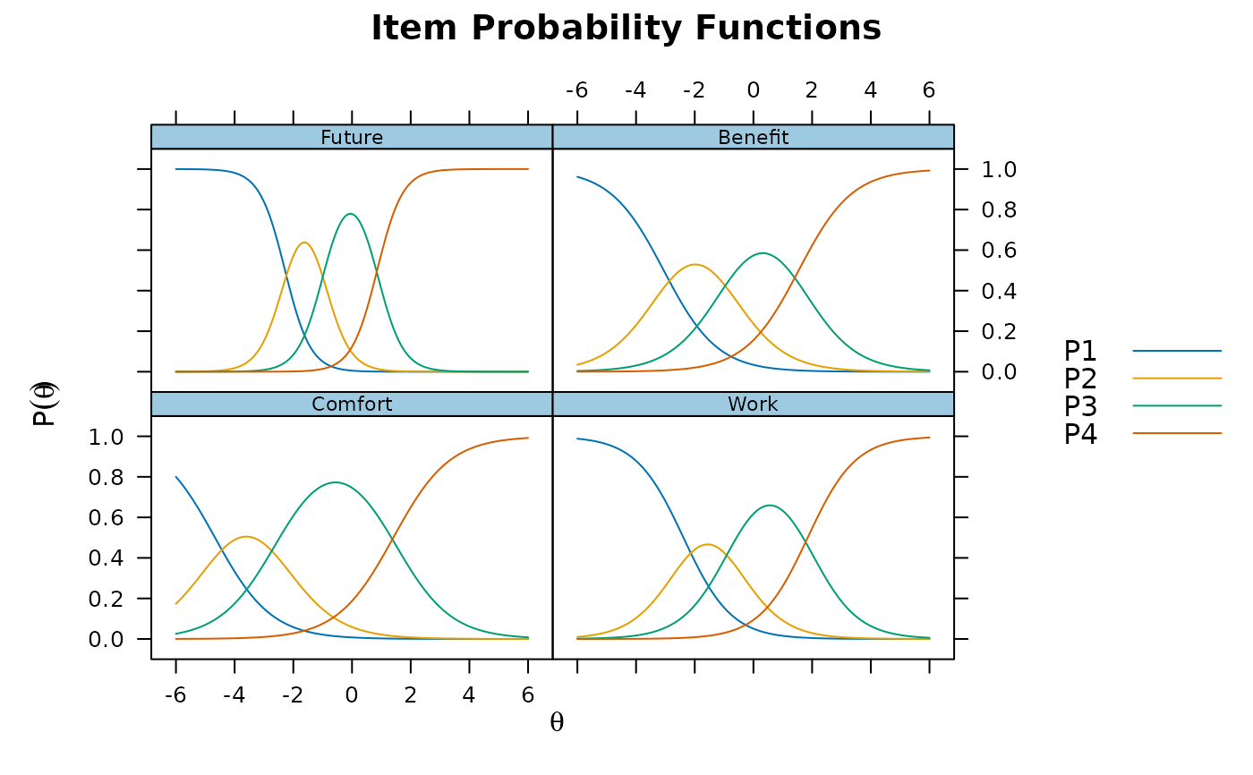plot(pmod1, type = 'itemscore')

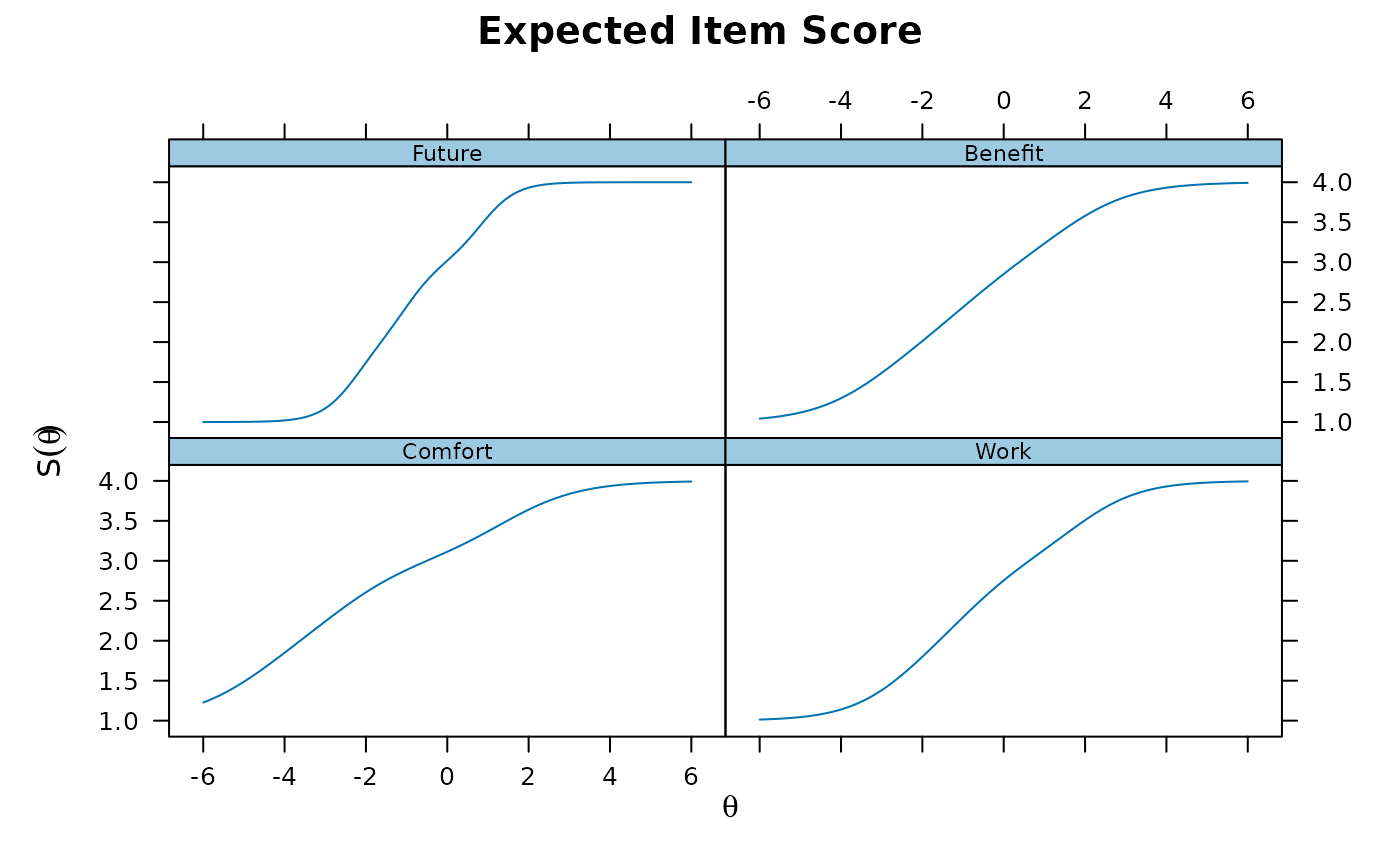summary(pmod1)
#>            F1    h2
#> Comfort 0.522 0.273
#> Work    0.584 0.342
#> Future  0.803 0.645
#> Benefit 0.541 0.293
#> 
#> SS loadings:  1.552 
#> Proportion Var:  0.388 
#> 
#> Factor correlations: 
#> 
#>    F1
#> F1  1

# Constrain all slopes to be equal with the constrain = list() input or mirt.model() syntax
# first obtain parameter index
values <- mirt(Science,1, pars = 'values')
values #note that slopes are numbered 1,5,9,13, or index with values$parnum[values$name == 'a1']
#>    group    item     class   name parnum  value lbound ubound   est const
#> 1    all Comfort    graded     a1      1  0.851   -Inf    Inf  TRUE  none
#> 2    all Comfort    graded     d1      2  4.390   -Inf    Inf  TRUE  none
#> 3    all Comfort    graded     d2      3  2.583   -Inf    Inf  TRUE  none
#> 4    all Comfort    graded     d3      4 -1.471   -Inf    Inf  TRUE  none
#> 5    all    Work    graded     a1      5  0.851   -Inf    Inf  TRUE  none
#> 6    all    Work    graded     d1      6  2.707   -Inf    Inf  TRUE  none
#> 7    all    Work    graded     d2      7  0.842   -Inf    Inf  TRUE  none
#> 8    all    Work    graded     d3      8 -2.120   -Inf    Inf  TRUE  none
#> 9    all  Future    graded     a1      9  0.851   -Inf    Inf  TRUE  none
#> 10   all  Future    graded     d1     10  3.543   -Inf    Inf  TRUE  none
#> 11   all  Future    graded     d2     11  1.522   -Inf    Inf  TRUE  none
#> 12   all  Future    graded     d3     12 -1.357   -Inf    Inf  TRUE  none
#> 13   all Benefit    graded     a1     13  0.851   -Inf    Inf  TRUE  none
#> 14   all Benefit    graded     d1     14  3.166   -Inf    Inf  TRUE  none
#> 15   all Benefit    graded     d2     15  0.982   -Inf    Inf  TRUE  none
#> 16   all Benefit    graded     d3     16 -1.661   -Inf    Inf  TRUE  none
#> 17   all   GROUP GroupPars MEAN_1     17  0.000   -Inf    Inf FALSE  none
#> 18   all   GROUP GroupPars COV_11     18  1.000      0    Inf FALSE  none
#>    nconst prior.type prior_1 prior_2
#> 1    none       none     NaN     NaN
#> 2    none       none     NaN     NaN
#> 3    none       none     NaN     NaN
#> 4    none       none     NaN     NaN
#> 5    none       none     NaN     NaN
#> 6    none       none     NaN     NaN
#> 7    none       none     NaN     NaN
#> 8    none       none     NaN     NaN
#> 9    none       none     NaN     NaN
#> 10   none       none     NaN     NaN
#> 11   none       none     NaN     NaN
#> 12   none       none     NaN     NaN
#> 13   none       none     NaN     NaN
#> 14   none       none     NaN     NaN
#> 15   none       none     NaN     NaN
#> 16   none       none     NaN     NaN
#> 17   none       none     NaN     NaN
#> 18   none       none     NaN     NaN
(pmod1_equalslopes <- mirt(Science, 1, constrain = list(c(1,5,9,13))))
#> 
#> 
#> Call:
#> mirt(data = Science, model = 1, constrain = list(c(1, 5, 9, 13)))
#> 
#> Full-information item factor analysis with 1 factor(s).
#> Converged within 1e-04 tolerance after 15 EM iterations.
#> mirt version: 1.44.5 
#> M-step optimizer: BFGS 
#> EM acceleration: Ramsay 
#> Number of rectangular quadrature: 61
#> Latent density type: Gaussian 
#> 
#> Log-likelihood = -1613.899
#> Estimated parameters: 13 
#> AIC = 3253.798
#> BIC = 3305.425; SABIC = 3264.176
#> G2 (242) = 223.62, p = 0.7959
#> RMSEA = 0, CFI = NaN, TLI = NaN
coef(pmod1_equalslopes)
#> $Comfort
#>        a1    d1    d2     d3
#> par 1.321 5.165 2.844 -1.587
#> 
#> $Work
#>        a1    d1    d2     d3
#> par 1.321 2.992 0.934 -2.319
#> 
#> $Future
#>        a1    d1    d2     d3
#> par 1.321 4.067 1.662 -1.488
#> 
#> $Benefit
#>        a1   d1    d2     d3
#> par 1.321 3.55 1.057 -1.806
#> 
#> $GroupPars
#>     MEAN_1 COV_11
#> par      0      1
#> 

# using mirt.model syntax, constrain all item slopes to be equal
model <- 'F = 1-4
          CONSTRAIN = (1-4, a1)'
(pmod1_equalslopes <- mirt(Science, model))
#> 
#> 
#> Call:
#> mirt(data = Science, model = model)
#> 
#> Full-information item factor analysis with 1 factor(s).
#> Converged within 1e-04 tolerance after 15 EM iterations.
#> mirt version: 1.44.5 
#> M-step optimizer: BFGS 
#> EM acceleration: Ramsay 
#> Number of rectangular quadrature: 61
#> Latent density type: Gaussian 
#> 
#> Log-likelihood = -1613.899
#> Estimated parameters: 13 
#> AIC = 3253.798
#> BIC = 3305.425; SABIC = 3264.176
#> G2 (242) = 223.62, p = 0.7959
#> RMSEA = 0, CFI = NaN, TLI = NaN
coef(pmod1_equalslopes)
#> $Comfort
#>        a1    d1    d2     d3
#> par 1.321 5.165 2.844 -1.587
#> 
#> $Work
#>        a1    d1    d2     d3
#> par 1.321 2.992 0.934 -2.319
#> 
#> $Future
#>        a1    d1    d2     d3
#> par 1.321 4.067 1.662 -1.488
#> 
#> $Benefit
#>        a1   d1    d2     d3
#> par 1.321 3.55 1.057 -1.806
#> 
#> $GroupPars
#>     MEAN_1 COV_11
#> par      0      1
#> 

coef(pmod1_equalslopes)
#> $Comfort
#>        a1    d1    d2     d3
#> par 1.321 5.165 2.844 -1.587
#> 
#> $Work
#>        a1    d1    d2     d3
#> par 1.321 2.992 0.934 -2.319
#> 
#> $Future
#>        a1    d1    d2     d3
#> par 1.321 4.067 1.662 -1.488
#> 
#> $Benefit
#>        a1   d1    d2     d3
#> par 1.321 3.55 1.057 -1.806
#> 
#> $GroupPars
#>     MEAN_1 COV_11
#> par      0      1
#> 
anova(pmod1_equalslopes, pmod1) #significantly worse fit with almost all criteria
#>                        AIC    SABIC       HQ      BIC    logLik     X2 df     p
#> pmod1_equalslopes 3253.798 3264.176 3274.259 3305.425 -1613.899                
#> pmod1             3249.739 3262.512 3274.922 3313.279 -1608.870 10.059  3 0.018

pmod2 <- mirt(Science, 2)
#> 
summary(pmod2)
#> 
#> Rotation:  oblimin 
#> 
#> Rotated factor loadings: 
#> 
#>              F1      F2    h2
#> Comfort  0.6016  0.0312 0.382
#> Work    -0.0573  0.7971 0.592
#> Future   0.3302  0.5153 0.548
#> Benefit  0.7231 -0.0239 0.506
#> 
#> Rotated SS loadings:  0.997 0.902 
#> 
#> Factor correlations: 
#> 
#>       F1 F2
#> F1 1.000   
#> F2 0.511  1
plot(pmod2, rotate = 'oblimin')

itemplot(pmod2, 1, rotate = 'oblimin')

anova(pmod1, pmod2)
#>            AIC    SABIC       HQ      BIC    logLik     X2 df     p
#> pmod1 3249.739 3262.512 3274.922 3313.279 -1608.870                
#> pmod2 3241.938 3257.106 3271.843 3317.392 -1601.969 13.801  3 0.003

# unidimensional fit with a generalized partial credit and nominal model
(gpcmod <- mirt(Science, 1, 'gpcm'))
#> 
#> 
#> Call:
#> mirt(data = Science, model = 1, itemtype = "gpcm")
#> 
#> Full-information item factor analysis with 1 factor(s).
#> Converged within 1e-04 tolerance after 50 EM iterations.
#> mirt version: 1.44.5 
#> M-step optimizer: BFGS 
#> EM acceleration: Ramsay 
#> Number of rectangular quadrature: 61
#> Latent density type: Gaussian 
#> 
#> Log-likelihood = -1612.683
#> Estimated parameters: 16 
#> AIC = 3257.366
#> BIC = 3320.906; SABIC = 3270.139
#> G2 (239) = 221.19, p = 0.7896
#> RMSEA = 0, CFI = NaN, TLI = NaN
coef(gpcmod)
#> $Comfort
#>        a1 ak0 ak1 ak2 ak3 d0    d1    d2    d3
#> par 0.865   0   1   2   3  0 2.831 5.324 3.998
#> 
#> $Work
#>        a1 ak0 ak1 ak2 ak3 d0    d1    d2    d3
#> par 0.841   0   1   2   3  0 1.711 2.578 0.848
#> 
#> $Future
#>        a1 ak0 ak1 ak2 ak3 d0    d1    d2    d3
#> par 2.204   0   1   2   3  0 4.601 6.759 4.918
#> 
#> $Benefit
#>        a1 ak0 ak1 ak2 ak3 d0    d1    d2    d3
#> par 0.724   0   1   2   3  0 2.099 2.899 1.721
#> 
#> $GroupPars
#>     MEAN_1 COV_11
#> par      0      1
#> 

# for the nominal model the lowest and highest categories are assumed to be the
#  theoretically lowest and highest categories that related to the latent trait(s)
(nomod <- mirt(Science, 1, 'nominal'))
#> 
#> 
#> Call:
#> mirt(data = Science, model = 1, itemtype = "nominal")
#> 
#> Full-information item factor analysis with 1 factor(s).
#> Converged within 1e-04 tolerance after 71 EM iterations.
#> mirt version: 1.44.5 
#> M-step optimizer: BFGS 
#> EM acceleration: Ramsay 
#> Number of rectangular quadrature: 61
#> Latent density type: Gaussian 
#> 
#> Log-likelihood = -1608.455
#> Estimated parameters: 24 
#> AIC = 3264.91
#> BIC = 3360.22; SABIC = 3284.069
#> G2 (231) = 212.73, p = 0.8002
#> RMSEA = 0, CFI = NaN, TLI = NaN
coef(nomod) #ordering of ak values suggest that the items are indeed ordinal
#> $Comfort
#>        a1 ak0   ak1   ak2 ak3 d0    d1    d2    d3
#> par 1.008   0 1.541 1.999   3  0 3.639 5.905 4.533
#> 
#> $Work
#>        a1 ak0   ak1 ak2 ak3 d0    d1    d2    d3
#> par 0.841   0 0.689 1.5   3  0 1.464 2.326 0.325
#> 
#> $Future
#>        a1 ak0   ak1   ak2 ak3 d0    d1    d2    d3
#> par 2.041   0 0.762 1.861   3  0 3.668 5.868 3.949
#> 
#> $Benefit
#>        a1 ak0   ak1   ak2 ak3 d0    d1    d2    d3
#> par 0.779   0 1.036 1.742   3  0 2.144 2.911 1.621
#> 
#> $GroupPars
#>     MEAN_1 COV_11
#> par      0      1
#> 
anova(gpcmod, nomod)
#>             AIC    SABIC       HQ      BIC    logLik    X2 df    p
#> gpcmod 3257.366 3270.139 3282.549 3320.906 -1612.683              
#> nomod  3264.910 3284.069 3302.684 3360.220 -1608.455 8.456  8 0.39
itemplot(nomod, 3)


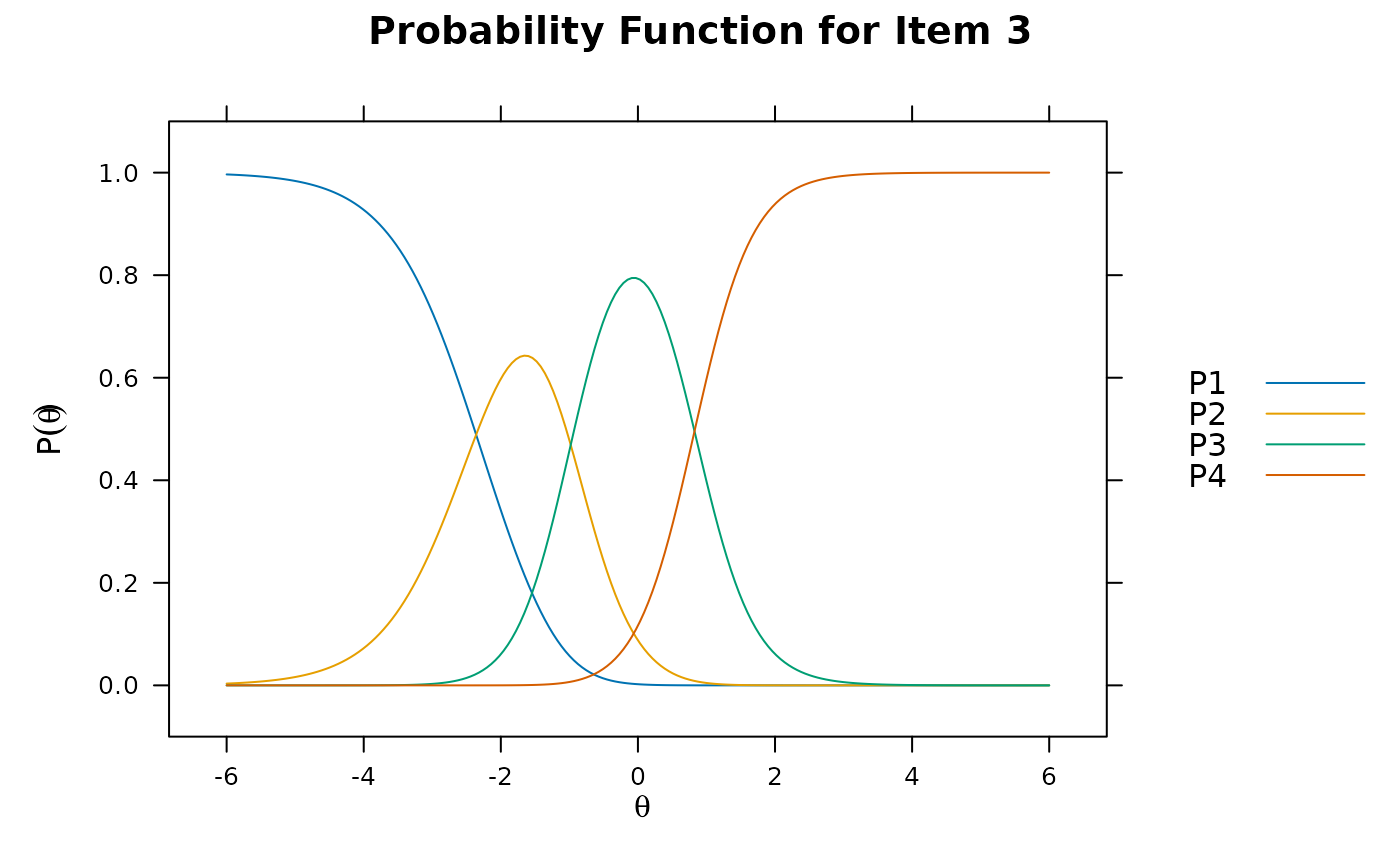# generalized graded unfolding model
(ggum <- mirt(Science, 1, 'ggum'))
#> 
#> 
#> Call:
#> mirt(data = Science, model = 1, itemtype = "ggum")
#> 
#> Full-information item factor analysis with 1 factor(s).
#> Converged within 1e-04 tolerance after 89 EM iterations.
#> mirt version: 1.44.5 
#> M-step optimizer: nlminb 
#> EM acceleration: Ramsay 
#> Number of rectangular quadrature: 61
#> Latent density type: Gaussian 
#> 
#> Log-likelihood = -1611.484
#> Estimated parameters: 20 
#> AIC = 3262.968
#> BIC = 3342.393; SABIC = 3278.934
#> G2 (235) = 218.79, p = 0.7687
#> RMSEA = 0, CFI = NaN, TLI = NaN
coef(ggum, simplify=TRUE)
#> $items
#>            a1    b1    t1    t2    t3
#> Comfort 0.824 3.478 6.826 6.475 1.780
#> Work    0.818 3.217 5.280 4.274 0.969
#> Future  2.241 2.800 4.888 3.774 1.961
#> Benefit 0.696 3.584 6.556 4.725 1.744
#> 
#> $means
#> F1 
#>  0 
#> 
#> $cov
#>    F1
#> F1  1
#> 
plot(ggum)

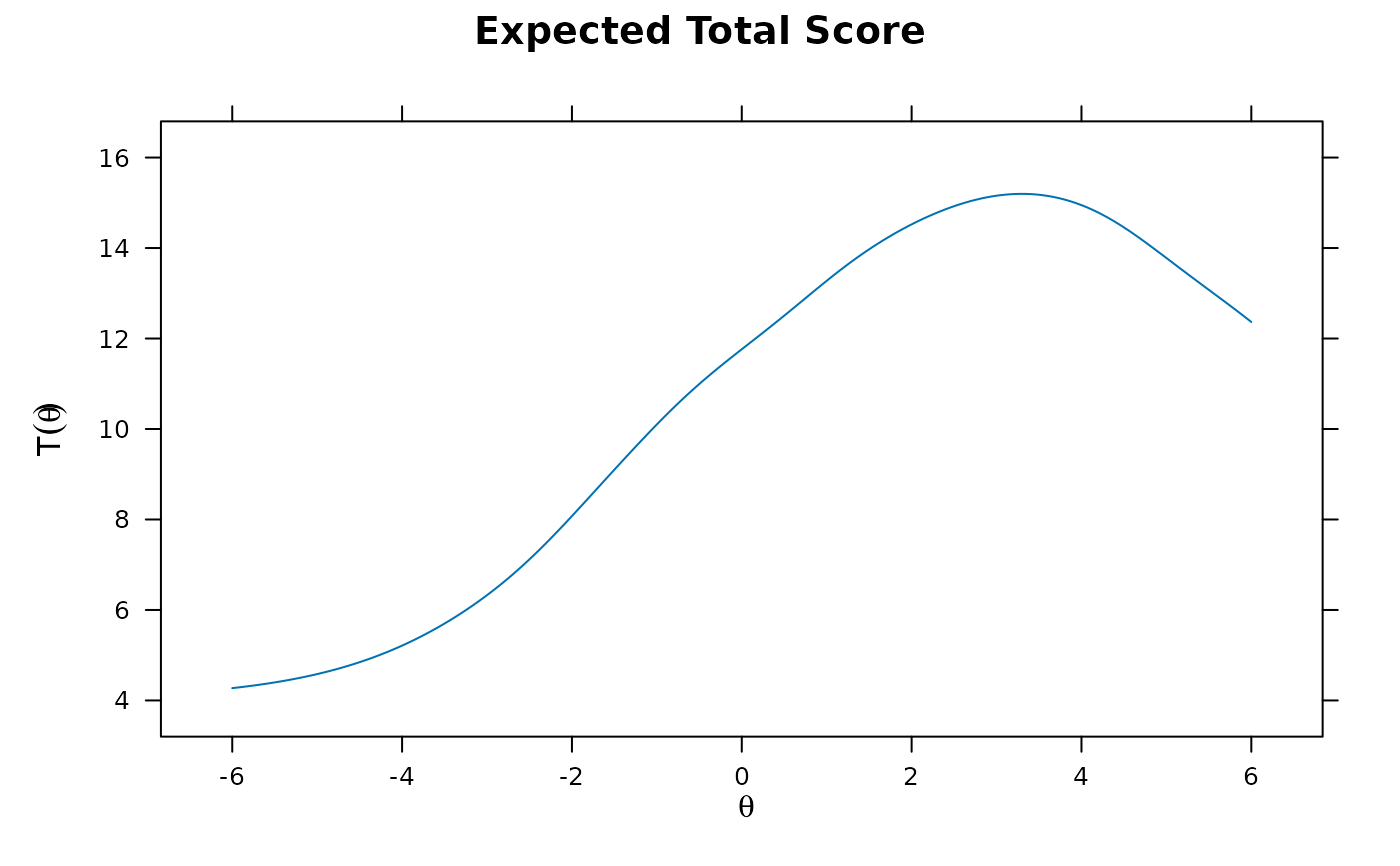plot(ggum, type = 'trace')

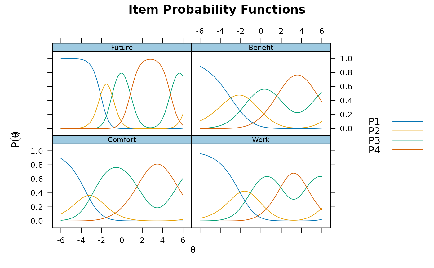plot(ggum, type = 'itemscore')


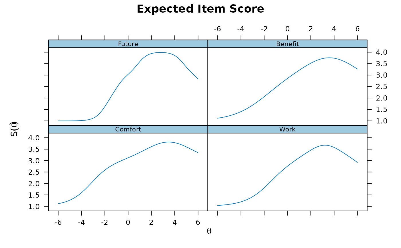# monotonic polyomial models
(monopoly <- mirt(Science, 1, 'monopoly'))
#> 
#> 
#> Call:
#> mirt(data = Science, model = 1, itemtype = "monopoly")
#> 
#> Full-information item factor analysis with 1 factor(s).
#> Converged within 1e-04 tolerance after 55 EM iterations.
#> mirt version: 1.44.5 
#> M-step optimizer: BFGS 
#> EM acceleration: Ramsay 
#> Number of rectangular quadrature: 61
#> Latent density type: Gaussian 
#> 
#> Log-likelihood = -1601.174
#> Estimated parameters: 24 
#> AIC = 3250.347
#> BIC = 3345.657; SABIC = 3269.506
#> G2 (231) = 198.17, p = 0.9424
#> RMSEA = 0, CFI = NaN, TLI = NaN
coef(monopoly, simplify=TRUE)
#> $items
#>          omega   xi1   xi2    xi3 alpha1   tau2
#> Comfort -1.431 2.911 2.218 -1.469 -0.934  0.728
#> Work    -0.412 1.378 0.698 -2.152 -0.499 -1.151
#> Future   0.833 4.988 2.259 -1.910  0.019 -8.472
#> Benefit -1.714 1.883 0.618 -1.389 -1.424  0.716
#> 
#> $means
#> F1 
#>  0 
#> 
#> $cov
#>    F1
#> F1  1
#> 
plot(monopoly)

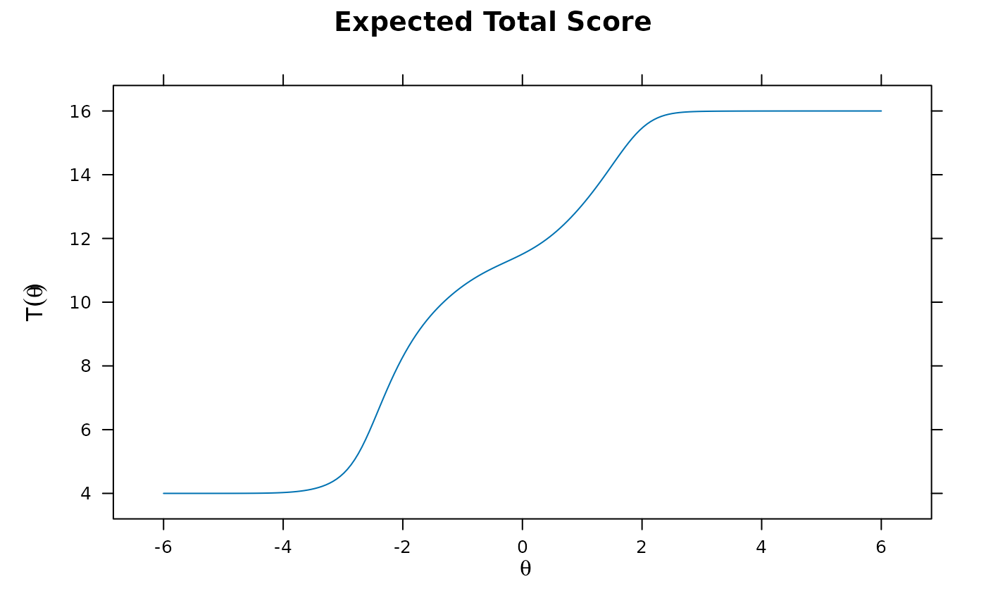plot(monopoly, type = 'trace')

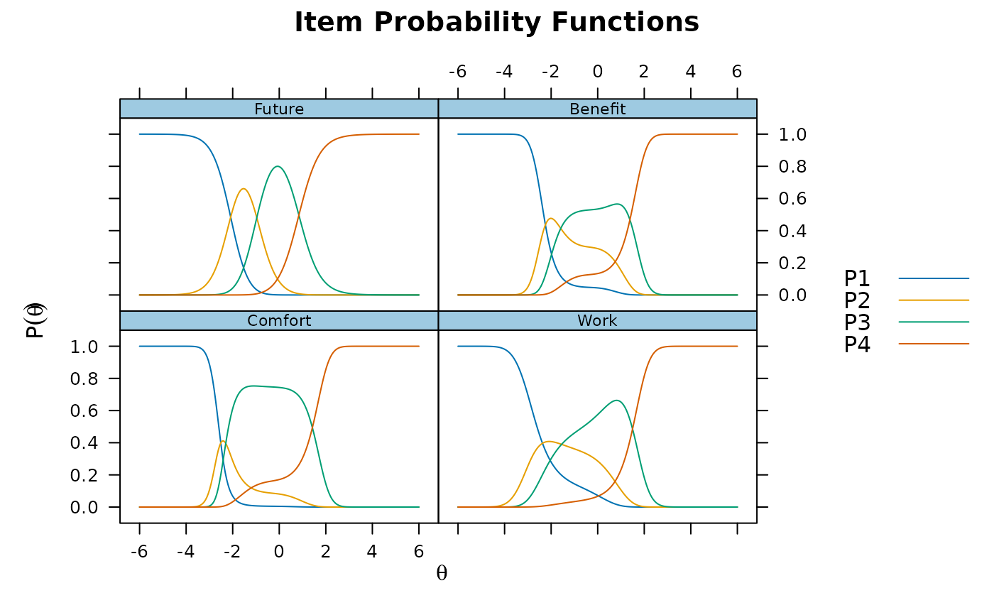plot(monopoly, type = 'itemscore')


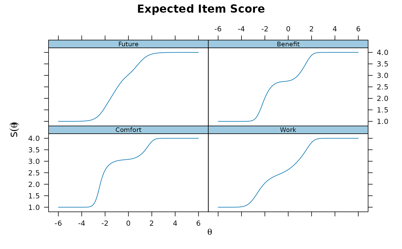# unipolar IRT model
unimod <- mirt(Science, itemtype = 'ULL')
#> 
coef(unimod, simplify=TRUE)
#> $items
#>          eta1 log_lambda1 log_lambda2 log_lambda3
#> Comfort 1.175       4.776       2.299      -1.709
#> Work    1.618       2.533       0.554      -2.736
#> Future  2.801       4.030       1.525      -2.594
#> Benefit 1.319       3.020       0.681      -1.995
#> 
#> $GroupPars
#>     meanlog sdlog
#> par       0     1
#> 
plot(unimod)

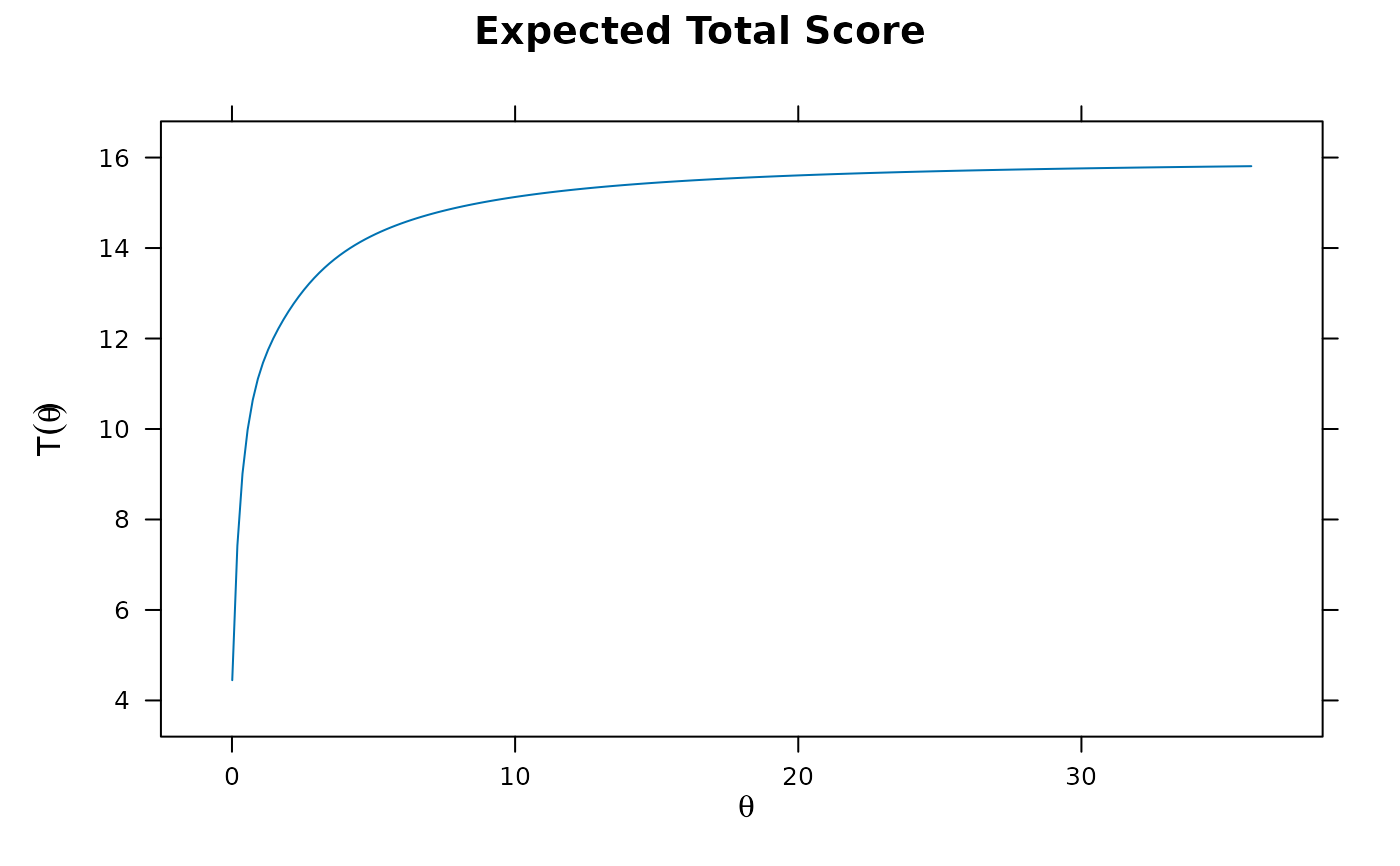plot(unimod, type = 'trace')

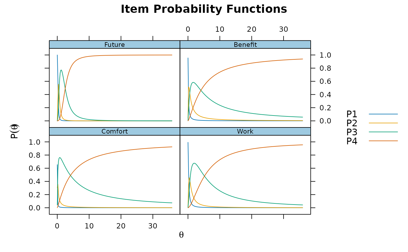itemplot(unimod, 1)


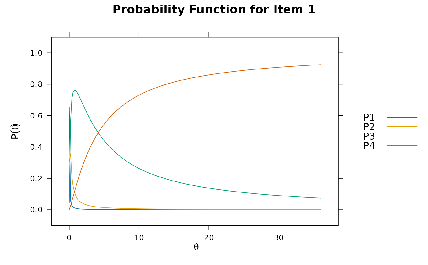# following use the correct log-normal density for latent trait
itemfit(unimod)
#>      item   S_X2 df.S_X2 RMSEA.S_X2 p.S_X2
#> 1 Comfort  5.664       6      0.000  0.462
#> 2    Work 10.136       8      0.026  0.256
#> 3  Future 19.477       8      0.061  0.013
#> 4 Benefit 12.106      11      0.016  0.356
M2(unimod, type = 'C2')
#>             M2 df            p     RMSEA    RMSEA_5  RMSEA_95     SRMSR
#> stats 18.69535  2 8.716799e-05 0.1461148 0.09026025 0.2096111 0.0786373
#>             TLI       CFI
#> stats 0.7376985 0.9125662
fs <- fscores(unimod)
hist(fs, 20)

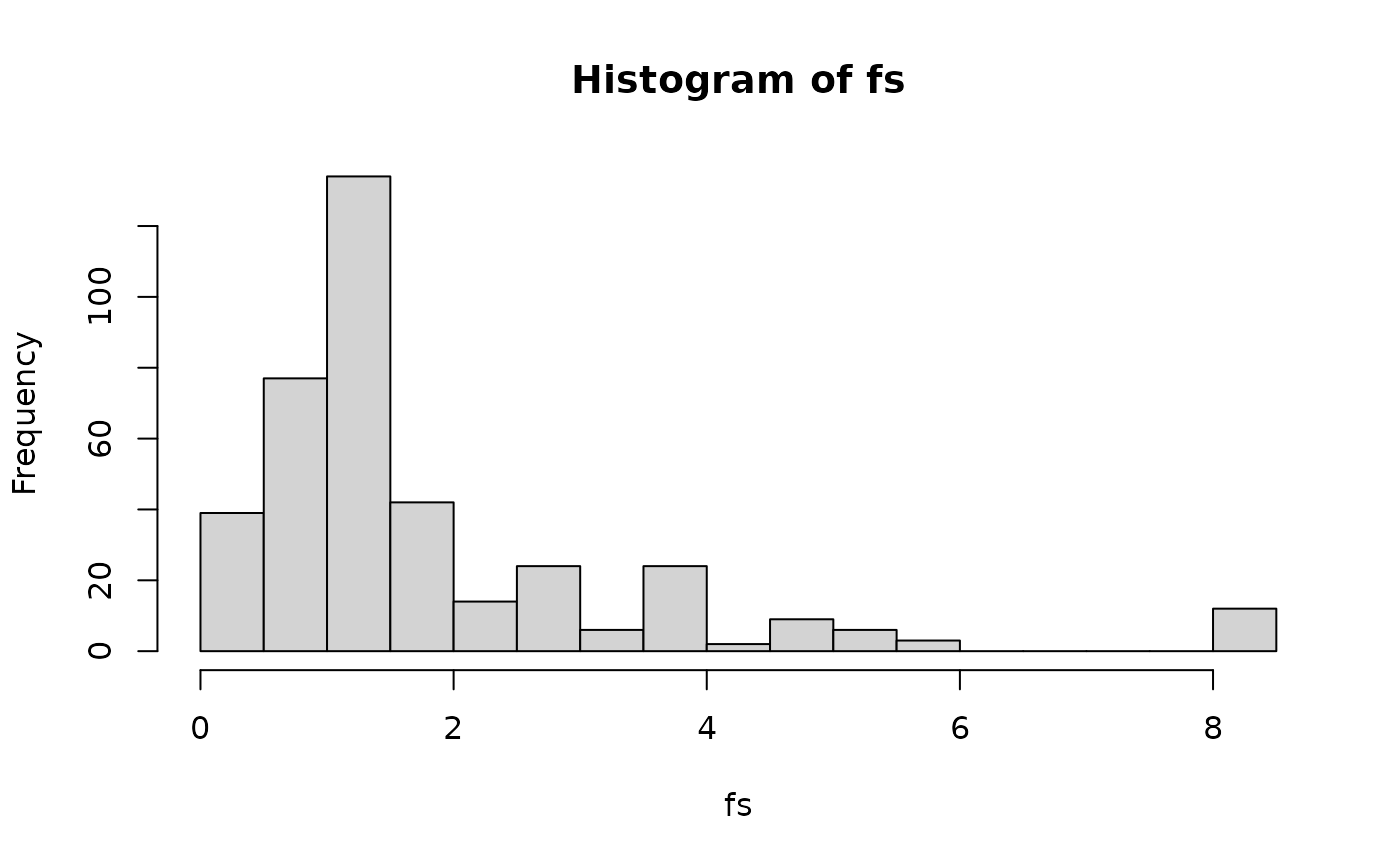fscores(unimod, method = 'EAPsum', full.scores = FALSE)
#>       df     X2 p.X2 SEM.alpha rxx.alpha rxx_F1
#> stats 10 33.926    0     1.305     0.658  0.531
#> 
#>    Sum.Scores    F1 SE_F1 observed expected std.res
#> 4           4 0.138 0.153        2    0.127   5.251
#> 5           5 0.304 0.088        1    0.766   0.267
#> 6           6 0.328 0.084        2    4.339   1.123
#> 7           7 0.352 0.126        1   13.909   3.461
#> 8           8 0.407 0.199       11   27.739   3.178
#> 9           9 0.530 0.305       32   40.624   1.353
#> 10         10 0.748 0.440       58   52.271   0.792
#> 11         11 1.053 0.604       70   63.507   0.815
#> 12         12 1.478 0.845       91   68.879   2.665
#> 13         13 2.164 1.282       56   54.418   0.214
#> 14         14 3.299 2.001       36   36.187   0.031
#> 15         15 5.109 3.236       20   20.821   0.180
#> 16         16 8.222 5.298       12    8.414   1.236

## example applying survey weights.
# weight the first half of the cases to be more representative of population
survey.weights <- c(rep(2, nrow(Science)/2), rep(1, nrow(Science)/2))
survey.weights <- survey.weights/sum(survey.weights) * nrow(Science)
unweighted <- mirt(Science, 1)
#> 
weighted <- mirt(Science, 1, survey.weights=survey.weights)
#> 

###########
# empirical dimensionality testing that includes 'guessing'

data(SAT12)
data <- key2binary(SAT12,
  key = c(1,4,5,2,3,1,2,1,3,1,2,4,2,1,5,3,4,4,1,4,3,3,4,1,3,5,1,3,1,5,4,5))
itemstats(data)
#> $overall
#>    N mean_total.score sd_total.score ave.r  sd.r alpha SEM.alpha
#>  600           18.202          5.054 0.108 0.075 0.798     2.272
#> 
#> $itemstats
#>           N  mean    sd total.r total.r_if_rm alpha_if_rm
#> Item.1  600 0.283 0.451   0.380         0.300       0.793
#> Item.2  600 0.568 0.496   0.539         0.464       0.785
#> Item.3  600 0.280 0.449   0.446         0.371       0.789
#> Item.4  600 0.378 0.485   0.325         0.235       0.796
#> Item.5  600 0.620 0.486   0.424         0.340       0.791
#> Item.6  600 0.160 0.367   0.414         0.351       0.791
#> Item.7  600 0.760 0.427   0.366         0.289       0.793
#> Item.8  600 0.202 0.402   0.307         0.233       0.795
#> Item.9  600 0.885 0.319   0.189         0.127       0.798
#> Item.10 600 0.422 0.494   0.465         0.383       0.789
#> Item.11 600 0.983 0.128   0.181         0.156       0.797
#> Item.12 600 0.415 0.493   0.173         0.076       0.803
#> Item.13 600 0.662 0.474   0.438         0.358       0.790
#> Item.14 600 0.723 0.448   0.411         0.333       0.791
#> Item.15 600 0.817 0.387   0.393         0.325       0.792
#> Item.16 600 0.413 0.493   0.367         0.278       0.794
#> Item.17 600 0.963 0.188   0.238         0.202       0.796
#> Item.18 600 0.352 0.478   0.576         0.508       0.783
#> Item.19 600 0.548 0.498   0.401         0.314       0.792
#> Item.20 600 0.873 0.333   0.376         0.318       0.792
#> Item.21 600 0.915 0.279   0.190         0.136       0.798
#> Item.22 600 0.935 0.247   0.284         0.238       0.795
#> Item.23 600 0.313 0.464   0.338         0.253       0.795
#> Item.24 600 0.728 0.445   0.422         0.346       0.791
#> Item.25 600 0.375 0.485   0.383         0.297       0.793
#> Item.26 600 0.460 0.499   0.562         0.489       0.783
#> Item.27 600 0.862 0.346   0.425         0.367       0.791
#> Item.28 600 0.530 0.500   0.465         0.383       0.789
#> Item.29 600 0.340 0.474   0.407         0.324       0.791
#> Item.30 600 0.440 0.497   0.255         0.159       0.799
#> Item.31 600 0.833 0.373   0.479         0.419       0.788
#> Item.32 600 0.162 0.368   0.110         0.037       0.802
#> 
#> $proportions
#>             0     1
#> Item.1  0.717 0.283
#> Item.2  0.432 0.568
#> Item.3  0.720 0.280
#> Item.4  0.622 0.378
#> Item.5  0.380 0.620
#> Item.6  0.840 0.160
#> Item.7  0.240 0.760
#> Item.8  0.798 0.202
#> Item.9  0.115 0.885
#> Item.10 0.578 0.422
#> Item.11 0.017 0.983
#> Item.12 0.585 0.415
#> Item.13 0.338 0.662
#> Item.14 0.277 0.723
#> Item.15 0.183 0.817
#> Item.16 0.587 0.413
#> Item.17 0.037 0.963
#> Item.18 0.648 0.352
#> Item.19 0.452 0.548
#> Item.20 0.127 0.873
#> Item.21 0.085 0.915
#> Item.22 0.065 0.935
#> Item.23 0.687 0.313
#> Item.24 0.272 0.728
#> Item.25 0.625 0.375
#> Item.26 0.540 0.460
#> Item.27 0.138 0.862
#> Item.28 0.470 0.530
#> Item.29 0.660 0.340
#> Item.30 0.560 0.440
#> Item.31 0.167 0.833
#> Item.32 0.838 0.162
#> 

mod1 <- mirt(data, 1)
#> 
extract.mirt(mod1, 'time') #time elapsed for each estimation component
#> TOTAL:   Data  Estep  Mstep     SE   Post 
#>  0.246  0.036  0.077  0.117  0.000  0.000 

# optionally use Newton-Raphson for (generally) faster convergence in the M-step's
mod1 <- mirt(data, 1, optimizer = 'NR')
#> 
extract.mirt(mod1, 'time')
#> TOTAL:   Data  Estep  Mstep     SE   Post 
#>  0.226  0.052  0.083  0.070  0.000  0.001 

mod2 <- mirt(data, 2, optimizer = 'NR')
#> 
#> Warning: EM cycles terminated after 500 iterations.
# difficulty converging with reduced quadpts, reduce TOL
mod3 <- mirt(data, 3, TOL = .001, optimizer = 'NR')
#> 
anova(mod1,mod2)
#>           AIC    SABIC       HQ      BIC    logLik     X2 df p
#> mod1 19105.91 19184.13 19215.46 19387.31 -9488.955            
#> mod2 19073.92 19190.03 19236.53 19491.63 -9441.963 93.985 31 0
anova(mod2, mod3) #negative AIC, 2 factors probably best
#>           AIC    SABIC       HQ      BIC    logLik     X2 df     p
#> mod2 19073.92 19190.03 19236.53 19491.63 -9441.963                
#> mod3 19080.18 19232.96 19294.13 19629.80 -9415.090 53.744 30 0.005

# same as above, but using the QMCEM method for generally better accuracy in mod3
mod3 <- mirt(data, 3, method = 'QMCEM', TOL = .001, optimizer = 'NR')
#> 
anova(mod2, mod3)
#>           AIC    SABIC       HQ      BIC    logLik     X2 df     p
#> mod2 19073.92 19190.03 19236.53 19491.63 -9441.963                
#> mod3 19081.58 19234.36 19295.54 19631.20 -9415.792 52.342 30 0.007

# with fixed guessing parameters
mod1g <- mirt(data, 1, guess = .1)
#> 
coef(mod1g)
#> $Item.1
#>        a1      d   g u
#> par 1.211 -1.737 0.1 1
#> 
#> $Item.2
#>       a1     d   g u
#> par 1.78 0.147 0.1 1
#> 
#> $Item.3
#>       a1    d   g u
#> par 1.91 -2.2 0.1 1
#> 
#> $Item.4
#>        a1      d   g u
#> par 0.833 -0.944 0.1 1
#> 
#> $Item.5
#>        a1     d   g u
#> par 1.089 0.399 0.1 1
#> 
#> $Item.6
#>        a1      d   g u
#> par 3.265 -5.212 0.1 1
#> 
#> $Item.7
#>       a1     d   g u
#> par 1.02 1.224 0.1 1
#> 
#> $Item.8
#>        a1      d   g u
#> par 1.639 -2.977 0.1 1
#> 
#> $Item.9
#>       a1     d   g u
#> par 0.49 2.007 0.1 1
#> 
#> $Item.10
#>        a1      d   g u
#> par 1.257 -0.756 0.1 1
#> 
#> $Item.11
#>       a1    d   g u
#> par 1.68 5.18 0.1 1
#> 
#> $Item.12
#>        a1      d   g u
#> par 0.191 -0.625 0.1 1
#> 
#> $Item.13
#>        a1     d   g u
#> par 1.147 0.654 0.1 1
#> 
#> $Item.14
#>        a1     d   g u
#> par 1.099 1.008 0.1 1
#> 
#> $Item.15
#>        a1    d   g u
#> par 1.337 1.79 0.1 1
#> 
#> $Item.16
#>        a1      d   g u
#> par 0.923 -0.744 0.1 1
#> 
#> $Item.17
#>        a1     d   g u
#> par 1.519 4.077 0.1 1
#> 
#> $Item.18
#>        a1      d   g u
#> par 2.585 -1.749 0.1 1
#> 
#> $Item.19
#>       a1      d   g u
#> par 0.91 -0.002 0.1 1
#> 
#> $Item.20
#>        a1     d   g u
#> par 1.485 2.438 0.1 1
#> 
#> $Item.21
#>        a1     d   g u
#> par 0.616 2.407 0.1 1
#> 
#> $Item.22
#>        a1     d   g u
#> par 1.429 3.291 0.1 1
#> 
#> $Item.23
#>       a1      d   g u
#> par 0.96 -1.393 0.1 1
#> 
#> $Item.24
#>        a1     d   g u
#> par 1.282 1.099 0.1 1
#> 
#> $Item.25
#>        a1  d   g u
#> par 1.028 -1 0.1 1
#> 
#> $Item.26
#>        a1      d   g u
#> par 2.059 -0.658 0.1 1
#> 
#> $Item.27
#>        a1     d   g u
#> par 1.839 2.564 0.1 1
#> 
#> $Item.28
#>        a1      d   g u
#> par 1.222 -0.095 0.1 1
#> 
#> $Item.29
#>        a1      d   g u
#> par 1.281 -1.357 0.1 1
#> 
#> $Item.30
#>        a1      d   g u
#> par 0.444 -0.521 0.1 1
#> 
#> $Item.31
#>        a1     d   g u
#> par 2.476 2.697 0.1 1
#> 
#> $Item.32
#>        a1      d   g u
#> par 0.461 -2.742 0.1 1
#> 
#> $GroupPars
#>     MEAN_1 COV_11
#> par      0      1
#> 

###########
# graded rating scale example

# make some data
set.seed(1234)
a <- matrix(rep(1, 10))
d <- matrix(c(1,0.5,-.5,-1), 10, 4, byrow = TRUE)
c <- seq(-1, 1, length.out=10)
data <- simdata(a, d + c, 2000, itemtype = rep('graded',10))
itemstats(data)
#> $overall
#>     N mean_total.score sd_total.score ave.r  sd.r alpha SEM.alpha
#>  2000           20.196           8.33 0.203 0.027 0.719     4.419
#> 
#> $itemstats
#>            N  mean    sd total.r total.r_if_rm alpha_if_rm
#> Item_1  2000 1.284 1.510   0.512         0.359       0.700
#> Item_2  2000 1.427 1.544   0.529         0.375       0.697
#> Item_3  2000 1.592 1.584   0.545         0.389       0.695
#> Item_4  2000 1.774 1.586   0.538         0.381       0.696
#> Item_5  2000 1.910 1.607   0.539         0.380       0.696
#> Item_6  2000 2.124 1.606   0.533         0.373       0.697
#> Item_7  2000 2.284 1.598   0.520         0.359       0.700
#> Item_8  2000 2.420 1.583   0.578         0.430       0.688
#> Item_9  2000 2.606 1.543   0.530         0.377       0.697
#> Item_10 2000 2.776 1.491   0.495         0.342       0.702
#> 
#> $proportions
#>             0     1     2     3     4
#> Item_1  0.500 0.096 0.182 0.065 0.158
#> Item_2  0.450 0.108 0.197 0.059 0.187
#> Item_3  0.407 0.108 0.182 0.092 0.212
#> Item_4  0.346 0.111 0.212 0.085 0.246
#> Item_5  0.319 0.102 0.211 0.086 0.281
#> Item_6  0.269 0.097 0.205 0.099 0.330
#> Item_7  0.244 0.073 0.211 0.101 0.372
#> Item_8  0.216 0.074 0.195 0.106 0.410
#> Item_9  0.175 0.072 0.196 0.083 0.473
#> Item_10 0.150 0.059 0.174 0.102 0.516
#> 

mod1 <- mirt(data, 1)
#> 
mod2 <- mirt(data, 1, itemtype = 'grsm')
#> 
coef(mod2)
#> $Item_1
#>        a1    b1     b2     b3     b4 c
#> par 0.959 0.001 -0.507 -1.541 -2.032 0
#> 
#> $Item_2
#>        a1    b1     b2     b3     b4     c
#> par 0.987 0.001 -0.507 -1.541 -2.032 0.235
#> 
#> $Item_3
#>        a1    b1     b2     b3     b4     c
#> par 0.994 0.001 -0.507 -1.541 -2.032 0.457
#> 
#> $Item_4
#>        a1    b1     b2     b3     b4     c
#> par 1.027 0.001 -0.507 -1.541 -2.032 0.728
#> 
#> $Item_5
#>        a1    b1     b2     b3     b4     c
#> par 0.995 0.001 -0.507 -1.541 -2.032 0.895
#> 
#> $Item_6
#>        a1    b1     b2     b3     b4     c
#> par 0.987 0.001 -0.507 -1.541 -2.032 1.179
#> 
#> $Item_7
#>        a1    b1     b2     b3     b4     c
#> par 0.957 0.001 -0.507 -1.541 -2.032 1.404
#> 
#> $Item_8
#>       a1    b1     b2     b3     b4     c
#> par 1.04 0.001 -0.507 -1.541 -2.032 1.578
#> 
#> $Item_9
#>        a1    b1     b2     b3     b4     c
#> par 0.964 0.001 -0.507 -1.541 -2.032 1.878
#> 
#> $Item_10
#>        a1    b1     b2     b3     b4     c
#> par 0.947 0.001 -0.507 -1.541 -2.032 2.136
#> 
#> $GroupPars
#>     MEAN_1 COV_11
#> par      0      1
#> 
anova(mod2, mod1) #not sig, mod2 should be preferred
#>           AIC    SABIC       HQ      BIC    logLik     X2 df     p
#> mod2 55239.72 55295.47 55287.03 55368.55 -27596.86                
#> mod1 55252.05 55373.25 55354.88 55532.10 -27576.03 41.671 27 0.035
itemplot(mod2, 1)

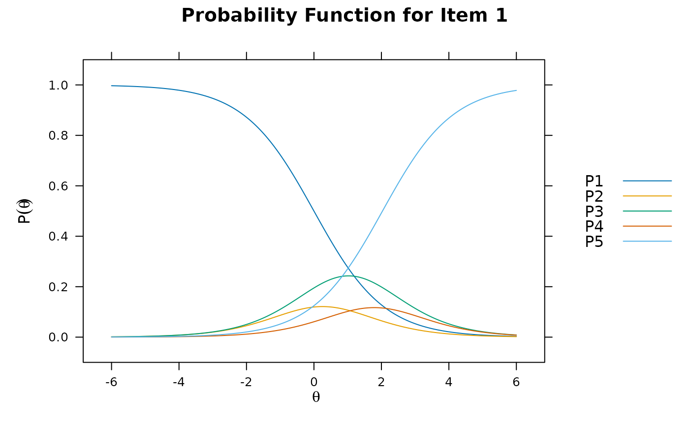itemplot(mod2, 5)

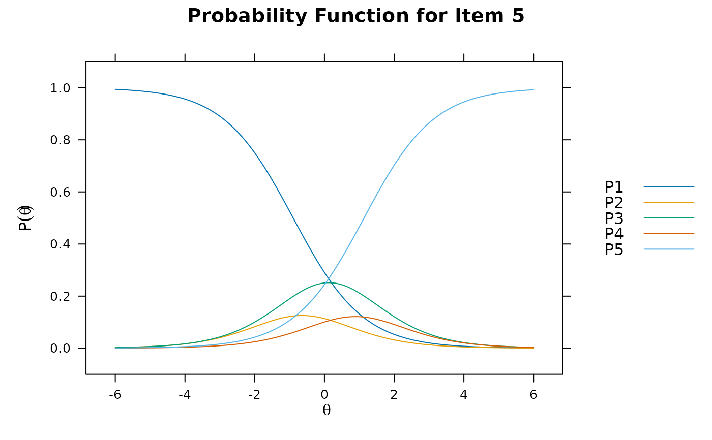itemplot(mod2, 10)


###########
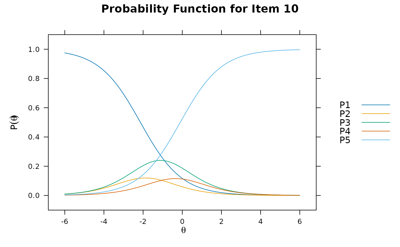# 2PL nominal response model example (Suh and Bolt, 2010)
data(SAT12)
SAT12[SAT12 == 8] <- NA #set 8 as a missing value
head(SAT12)
#>   Item.1 Item.2 Item.3 Item.4 Item.5 Item.6 Item.7 Item.8 Item.9 Item.10
#> 1      1      4      5      2      3      1      2      1      3       1
#> 2      3      4      2     NA      3      3      2     NA      3       1
#> 3      1      4      5      4      3      2      2      3      3       2
#> 4      2      4      4      2      3      3      2      4      3       2
#> 5      2      4      5      2      3      2      2      1      1       2
#> 6      1      4      3      1      3      2      2      3      3       1
#>   Item.11 Item.12 Item.13 Item.14 Item.15 Item.16 Item.17 Item.18 Item.19
#> 1       2       4       2       1       5       3       4       4       1
#> 2       2      NA       2       1       5       2       4       1       1
#> 3       2       1       3       1       5       5       4       1       3
#> 4       2       4       2       1       5       2       4       1       3
#> 5       2       4       2       1       5       4       4       5       1
#> 6       2       3       2       1       5       5       4       4       1
#>   Item.20 Item.21 Item.22 Item.23 Item.24 Item.25 Item.26 Item.27 Item.28
#> 1       4       3       3       4       1       3       5       1       3
#> 2       4       3       3      NA       1      NA       4       1       4
#> 3       4       3       3       1       1       3       4       1       3
#> 4       4       3       1       5       2       5       4       1       3
#> 5       4       3       3       3       1       1       5       1       3
#> 6       4       3       3       4       1       1       4       1       4
#>   Item.29 Item.30 Item.31 Item.32
#> 1       1       5       4       5
#> 2       5      NA       4      NA
#> 3       4       4       4       1
#> 4       4       2       4       2
#> 5       1       2       4       1
#> 6       2       3       4       3

# correct answer key
key <- c(1,4,5,2,3,1,2,1,3,1,2,4,2,1,5,3,4,4,1,4,3,3,4,1,3,5,1,3,1,5,4,5)
scoredSAT12 <- key2binary(SAT12, key)
mod0 <- mirt(scoredSAT12, 1)
#> 

# for first 5 items use 2PLNRM and nominal
scoredSAT12[,1:5] <- as.matrix(SAT12[,1:5])
mod1 <- mirt(scoredSAT12, 1, c(rep('nominal',5),rep('2PL', 27)))
#> 
mod2 <- mirt(scoredSAT12, 1, c(rep('2PLNRM',5),rep('2PL', 27)), key=key)
#> 
coef(mod0)$Item.1
#>            a1         d g u
#> par 0.8107167 -1.042366 0 1
coef(mod1)$Item.1
#>             a1 ak0       ak1      ak2      ak3 ak4 d0         d1         d2
#> par -0.8772035   0 0.5286601 1.116593 1.129494   4  0 -0.1909232 0.01878861
#>             d3       d4
#> par -0.1258261 -5.65218
coef(mod2)$Item.1
#>            a1        d g u ak0        ak1        ak2       ak3 d0        d1
#> par 0.8102548 -1.04233 0 1   0 -0.5653287 -0.5712706 -3.025613  0 0.2117761
#>             d2        d3
#> par 0.06919723 -5.309272
itemplot(mod0, 1)

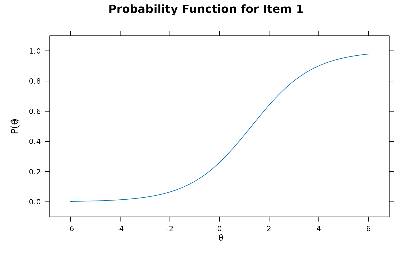itemplot(mod1, 1)

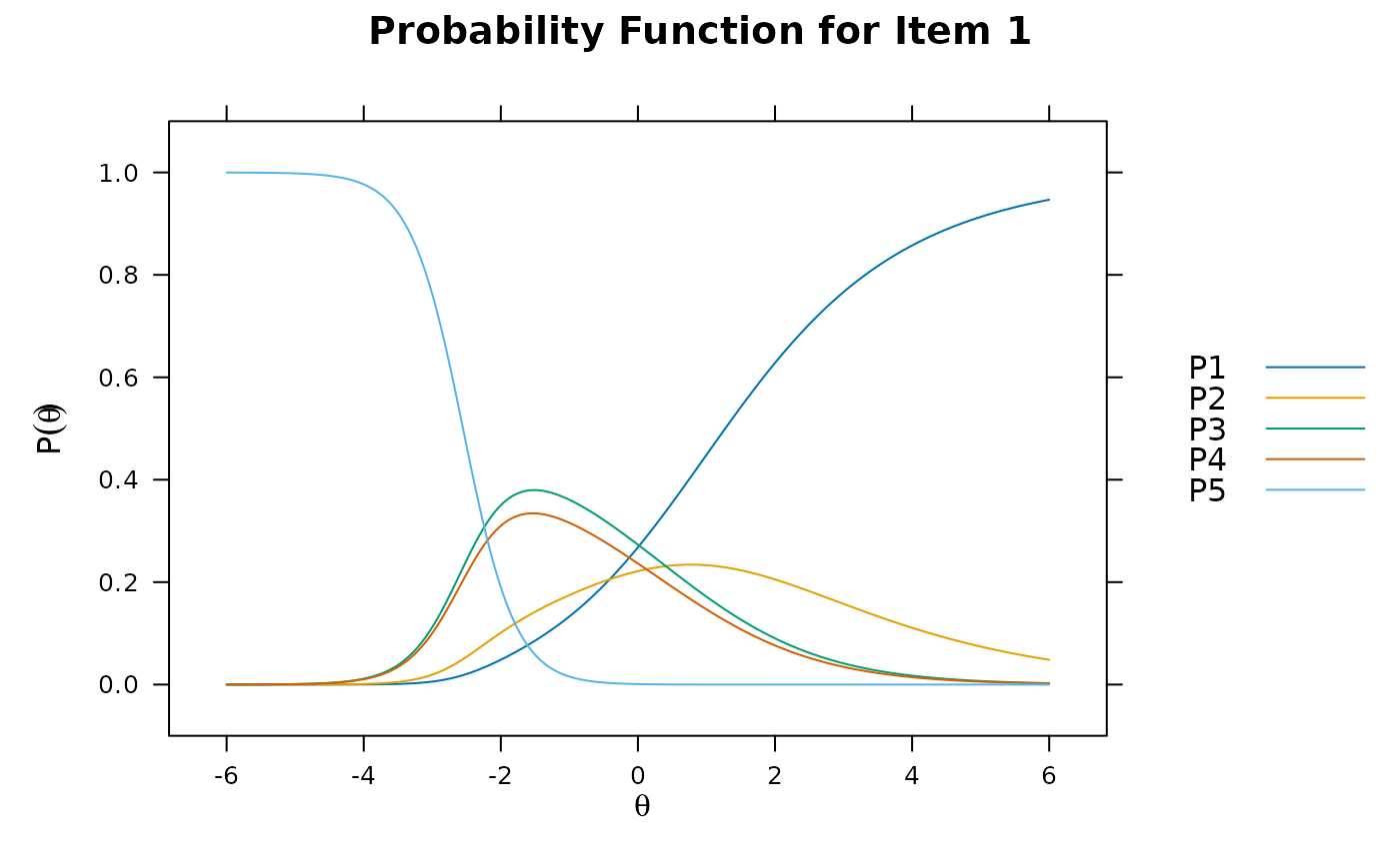itemplot(mod2, 1)


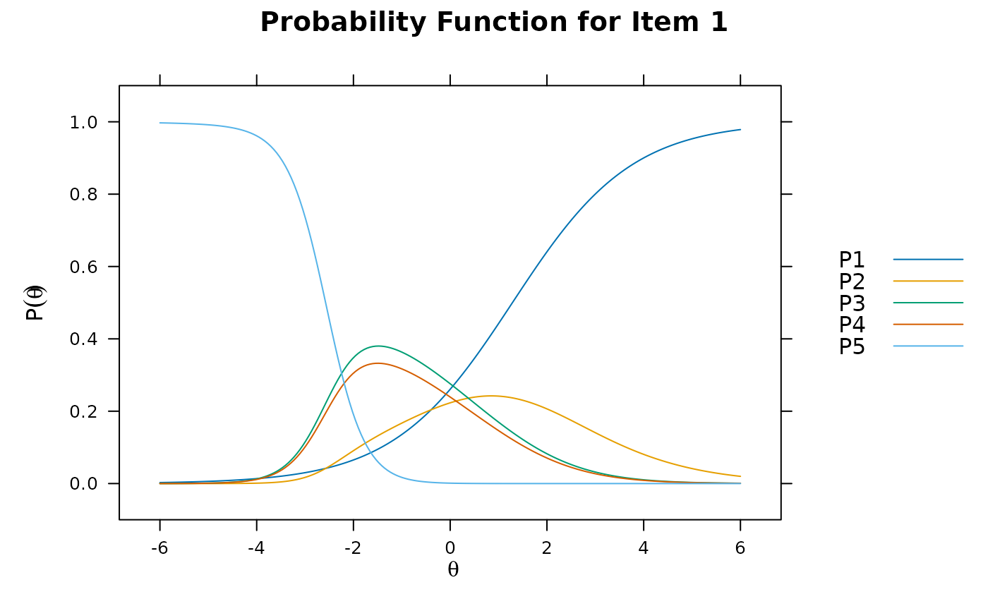# compare added information from distractors
Theta <- matrix(seq(-4,4,.01))
par(mfrow = c(2,3))
for(i in 1:5){
    info <- iteminfo(extract.item(mod0,i), Theta)
    info2 <- iteminfo(extract.item(mod2,i), Theta)
    plot(Theta, info2, type = 'l', main = paste('Information for item', i), ylab = 'Information')
    lines(Theta, info, col = 'red')
}
par(mfrow = c(1,1))


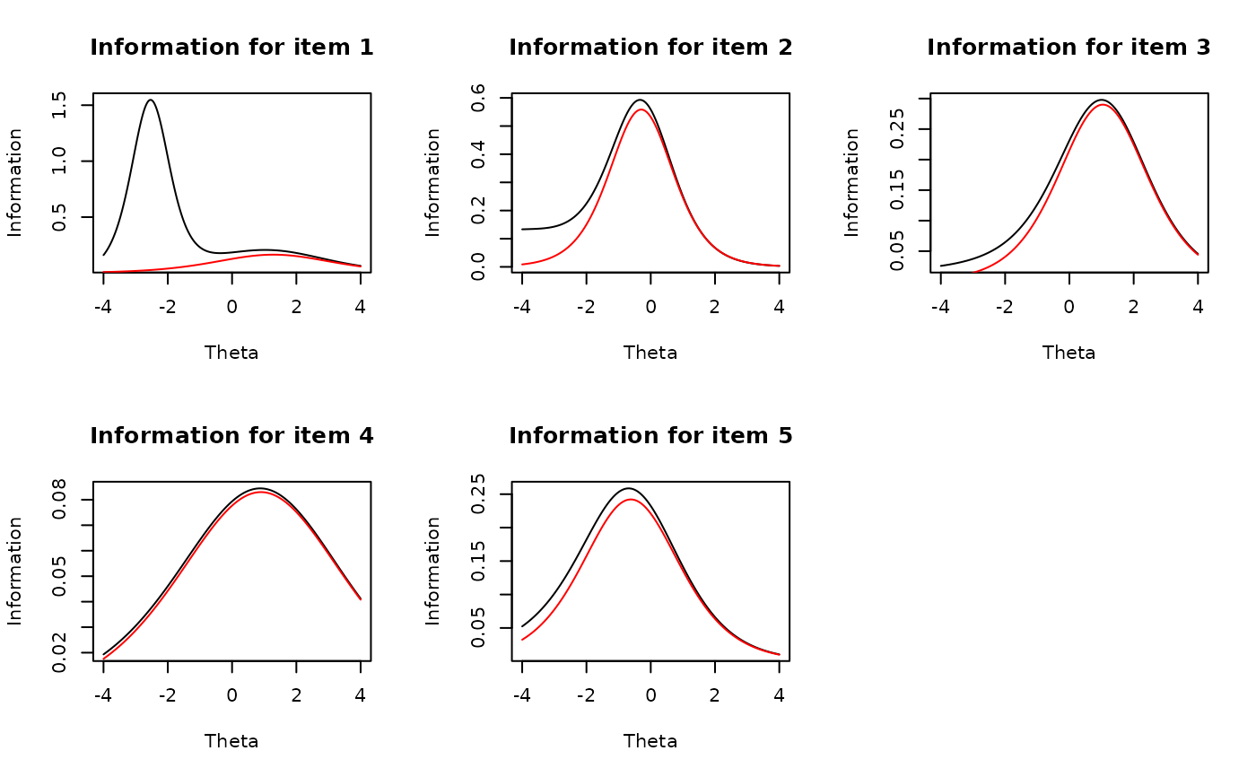# test information
plot(Theta, testinfo(mod2, Theta), type = 'l', main = 'Test information', ylab = 'Information')
lines(Theta, testinfo(mod0, Theta), col = 'red')


###########
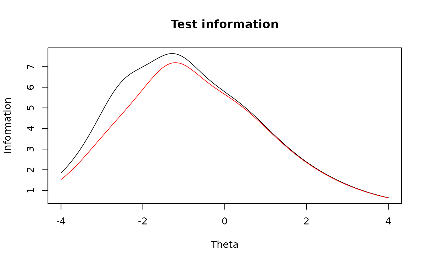# using the MH-RM algorithm
data(LSAT7)
fulldata <- expand.table(LSAT7)
(mod1 <- mirt(fulldata, 1, method = 'MHRM'))
#> , Max-Change = 0.0343, Max-Change = 0.0321, Max-Change = 0.0244, Max-Change = 0.0454, Max-Change = 0.0518, Max-Change = 0.0217, Max-Change = 0.0328, Max-Change = 0.0227, Max-Change = 0.0287, Max-Change = 0.0194, Max-Change = 0.0210, Max-Change = 0.0517, Max-Change = 0.0631, Max-Change = 0.0216, Max-Change = 0.0277, Max-Change = 0.0191, Max-Change = 0.0253, Max-Change = 0.0380, Max-Change = 0.0219, Max-Change = 0.0382, Max-Change = 0.0325, Max-Change = 0.0429, Max-Change = 0.0375, Max-Change = 0.0238, Max-Change = 0.0391, Max-Change = 0.0400, Max-Change = 0.0139, Max-Change = 0.0325, Max-Change = 0.0143, Max-Change = 0.0271, Max-Change = 0.0202, Max-Change = 0.0155, Max-Change = 0.0353, Max-Change = 0.0603, Max-Change = 0.0193, Max-Change = 0.0270, Max-Change = 0.0234, Max-Change = 0.0329, Max-Change = 0.0450, Max-Change = 0.0438, Max-Change = 0.0420, Max-Change = 0.0558, Max-Change = 0.0300, Max-Change = 0.0203, Max-Change = 0.0384, Max-Change = 0.0183, Max-Change = 0.0178, Max-Change = 0.0142, Max-Change = 0.0165, Max-Change = 0.0152, Max-Change = 0.0430, Max-Change = 0.0577, Max-Change = 0.0273, Max-Change = 0.0351, Max-Change = 0.0191, Max-Change = 0.0106, Max-Change = 0.0242, Max-Change = 0.0290, Max-Change = 0.0189, Max-Change = 0.0211, Max-Change = 0.0176, Max-Change = 0.0322, Max-Change = 0.0263, Max-Change = 0.0259, Max-Change = 0.0295, Max-Change = 0.0401, Max-Change = 0.0123, Max-Change = 0.0411, Max-Change = 0.0175, Max-Change = 0.0356, Max-Change = 0.0190, Max-Change = 0.0254, Max-Change = 0.0190, Max-Change = 0.0235, Max-Change = 0.0216, Max-Change = 0.0183, Max-Change = 0.0151, Max-Change = 0.0392, Max-Change = 0.0207, Max-Change = 0.0135, Max-Change = 0.0314, Max-Change = 0.0380, Max-Change = 0.0442, Max-Change = 0.0163, Max-Change = 0.0227, Max-Change = 0.0268, Max-Change = 0.0140, Max-Change = 0.0211, Max-Change = 0.0146, Max-Change = 0.0419, Max-Change = 0.0299, Max-Change = 0.0168, Max-Change = 0.0297, Max-Change = 0.0207, Max-Change = 0.0229, Max-Change = 0.0329, Max-Change = 0.0384, Max-Change = 0.0203, Max-Change = 0.0273, Max-Change = 0.0129, Max-Change = 0.0143, Max-Change = 0.0248, Max-Change = 0.0268, Max-Change = 0.0267, Max-Change = 0.0342, Max-Change = 0.0256, Max-Change = 0.0346, Max-Change = 0.0357, Max-Change = 0.0225, Max-Change = 0.0236, Max-Change = 0.0390, Max-Change = 0.0243, Max-Change = 0.0328, Max-Change = 0.0294, Max-Change = 0.0478, Max-Change = 0.0269, Max-Change = 0.0292, Max-Change = 0.0329, Max-Change = 0.0127, Max-Change = 0.0280, Max-Change = 0.0355, Max-Change = 0.0357, Max-Change = 0.0183, Max-Change = 0.0201, Max-Change = 0.0258, Max-Change = 0.0241, Max-Change = 0.0265, Max-Change = 0.0413, Max-Change = 0.0309, Max-Change = 0.0368, Max-Change = 0.0182, Max-Change = 0.0521, Max-Change = 0.0192, Max-Change = 0.0279, Max-Change = 0.0287, Max-Change = 0.0111, Max-Change = 0.0109, Max-Change = 0.0181, Max-Change = 0.0334, Max-Change = 0.0324, Max-Change = 0.0434, Max-Change = 0.0336, Max-Change = 0.0361, Max-Change = 0.0365, Max-Change = 0.0401, Max-Change = 0.0390, Max-Change = 0.0134, Max-Change = 0.0310, Max-Change = 0.0252, Max-Change = 0.0230, Max-Change = 0.0128, Max-Change = 0.0381, Max-Change = 0.0210, Max-Change = 0.0256, Max-Change = 0.0320, Max-Change = 0.0227, Max-Change = 0.0332, Max-Change = 0.0103, Max-Change = 0.0267, Max-Change = 0.0244, Max-Change = 0.0244, Max-Change = 0.0336, Max-Change = 0.0209, Max-Change = 0.0287, Max-Change = 0.0210, Max-Change = 0.0163, Max-Change = 0.0394, Max-Change = 0.0194, Max-Change = 0.0141, Max-Change = 0.0347, Max-Change = 0.0188, Max-Change = 0.0249, Max-Change = 0.0504, Max-Change = 0.0254, Max-Change = 0.0192, Max-Change = 0.0197, Max-Change = 0.0477, Max-Change = 0.0258, Max-Change = 0.0296, Max-Change = 0.0425, Max-Change = 0.0353, Max-Change = 0.0328, Max-Change = 0.0186, Max-Change = 0.0190, Max-Change = 0.0243, Max-Change = 0.0284, Max-Change = 0.0441, Max-Change = 0.0193, Max-Change = 0.0185, Max-Change = 0.0279, Max-Change = 0.0206, Max-Change = 0.0270, Max-Change = 0.0225, Max-Change = 0.0261, Max-Change = 0.0200, Max-Change = 0.0242, Max-Change = 0.0229, Max-Change = 0.0176, Max-Change = 0.0300, Max-Change = 0.0435, Max-Change = 0.0193, Max-Change = 0.0254, Max-Change = 0.0431, Max-Change = 0.0187, Max-Change = 0.0259, Max-Change = 0.0235, Max-Change = 0.0274, Max-Change = 0.0291, Max-Change = 0.0226, Max-Change = 0.0347, Max-Change = 0.0352, Max-Change = 0.0129, Max-Change = 0.0599, Max-Change = 0.0234, Max-Change = 0.0325, Max-Change = 0.0117, Max-Change = 0.0211, Max-Change = 0.0094, Max-Change = 0.0331, Max-Change = 0.0236, Max-Change = 0.0391, Max-Change = 0.0287, Max-Change = 0.0359, Max-Change = 0.0266, Max-Change = 0.0286, Max-Change = 0.0188, Max-Change = 0.0268, Max-Change = 0.0187, Max-Change = 0.0217, Max-Change = 0.0414, Max-Change = 0.0215, Max-Change = 0.0299, Max-Change = 0.0270, Max-Change = 0.0305, Max-Change = 0.0661, Max-Change = 0.0131, Max-Change = 0.0423, Max-Change = 0.0174, Max-Change = 0.0311, Max-Change = 0.0227, Max-Change = 0.0335, Max-Change = 0.0233, Max-Change = 0.0172, Max-Change = 0.0584, Max-Change = 0.0442, Max-Change = 0.0101, Max-Change = 0.0284, Max-Change = 0.0279, Max-Change = 0.0353, Max-Change = 0.0325, gam = 0.0000, Max-Change = 0.0000, gam = 0.1778, Max-Change = 0.0136, gam = 0.1057, Max-Change = 0.0187, gam = 0.0780, Max-Change = 0.0054, gam = 0.0629, Max-Change = 0.0068, gam = 0.0532, Max-Change = 0.0054, gam = 0.0464, Max-Change = 0.0051, gam = 0.0413, Max-Change = 0.0079, gam = 0.0374, Max-Change = 0.0091, gam = 0.0342, Max-Change = 0.0035, gam = 0.0316, Max-Change = 0.0049, gam = 0.0294, Max-Change = 0.0015, gam = 0.0276, Max-Change = 0.0042, gam = 0.0260, Max-Change = 0.0040, gam = 0.0246, Max-Change = 0.0085, gam = 0.0233, Max-Change = 0.0034, gam = 0.0222, Max-Change = 0.0031, gam = 0.0212, Max-Change = 0.0021, gam = 0.0203, Max-Change = 0.0027, gam = 0.0195, Max-Change = 0.0016, gam = 0.0188, Max-Change = 0.0026, gam = 0.0181, Max-Change = 0.0033, gam = 0.0175, Max-Change = 0.0036, gam = 0.0169, Max-Change = 0.0023, gam = 0.0164, Max-Change = 0.0019, gam = 0.0159, Max-Change = 0.0020, gam = 0.0154, Max-Change = 0.0024, gam = 0.0150, Max-Change = 0.0012, gam = 0.0146, Max-Change = 0.0021, gam = 0.0142, Max-Change = 0.0013, gam = 0.0139, Max-Change = 0.0034, gam = 0.0135, Max-Change = 0.0010, gam = 0.0132, Max-Change = 0.0017, gam = 0.0129, Max-Change = 0.0029, gam = 0.0126, Max-Change = 0.0019, gam = 0.0124, Max-Change = 0.0015, gam = 0.0121, Max-Change = 0.0030, gam = 0.0119, Max-Change = 0.0017, gam = 0.0116, Max-Change = 0.0006, gam = 0.0114, Max-Change = 0.0007, gam = 0.0112, Max-Change = 0.0013, gam = 0.0110, Max-Change = 0.0008, gam = 0.0108, Max-Change = 0.0011, gam = 0.0106, Max-Change = 0.0010, gam = 0.0104, Max-Change = 0.0014, gam = 0.0102, Max-Change = 0.0023, gam = 0.0101, Max-Change = 0.0025, gam = 0.0099, Max-Change = 0.0013, gam = 0.0098, Max-Change = 0.0014, gam = 0.0096, Max-Change = 0.0018, gam = 0.0095, Max-Change = 0.0012, gam = 0.0093, Max-Change = 0.0008, gam = 0.0092, Max-Change = 0.0009, gam = 0.0091, Max-Change = 0.0019, gam = 0.0089, Max-Change = 0.0030, gam = 0.0088, Max-Change = 0.0014, gam = 0.0087, Max-Change = 0.0004, gam = 0.0086, Max-Change = 0.0010, gam = 0.0085, Max-Change = 0.0009, gam = 0.0084, Max-Change = 0.0023, gam = 0.0082, Max-Change = 0.0013, gam = 0.0081, Max-Change = 0.0007, gam = 0.0080, Max-Change = 0.0006, gam = 0.0080, Max-Change = 0.0015, gam = 0.0079, Max-Change = 0.0006, gam = 0.0078, Max-Change = 0.0023, gam = 0.0077, Max-Change = 0.0007, gam = 0.0076, Max-Change = 0.0003, gam = 0.0075, Max-Change = 0.0014, gam = 0.0074, Max-Change = 0.0012, gam = 0.0073, Max-Change = 0.0009, gam = 0.0073, Max-Change = 0.0008, gam = 0.0072, Max-Change = 0.0006

#> 
#> Calculating log-likelihood...
#> 
#> Call:
#> mirt(data = fulldata, model = 1, method = "MHRM")
#> 
#> Full-information item factor analysis with 1 factor(s).
#> Converged within 0.001 tolerance after 73 MHRM iterations.
#> mirt version: 1.44.5 
#> M-step optimizer: NR1 
#> Latent density type: Gaussian 
#> Average MH acceptance ratio(s): 0.4 
#> 
#> Log-likelihood = -2659.472, SE = 0.018
#> Estimated parameters: 10 
#> AIC = 5338.944
#> BIC = 5388.022; SABIC = 5356.261
#> G2 (21) = 32.89, p = 0.0475
#> RMSEA = 0.024, CFI = NaN, TLI = NaN

# Confirmatory models

# simulate data
a <- matrix(c(
1.5,NA,
0.5,NA,
1.0,NA,
1.0,0.5,
 NA,1.5,
 NA,0.5,
 NA,1.0,
 NA,1.0),ncol=2,byrow=TRUE)

d <- matrix(c(
-1.0,NA,NA,
-1.5,NA,NA,
 1.5,NA,NA,
 0.0,NA,NA,
3.0,2.0,-0.5,
2.5,1.0,-1,
2.0,0.0,NA,
1.0,NA,NA),ncol=3,byrow=TRUE)

sigma <- diag(2)
sigma[1,2] <- sigma[2,1] <- .4
items <- c(rep('2PL',4), rep('graded',3), '2PL')
dataset <- simdata(a,d,2000,items,sigma)

# analyses
# CIFA for 2 factor crossed structure

model.1 <- '
  F1 = 1-4
  F2 = 4-8
  COV = F1*F2'

# compute model, and use parallel computation of the log-likelihood
if(interactive()) mirtCluster()
mod1 <- mirt(dataset, model.1, method = 'MHRM')
#> , Max-Change = 0.0465, Max-Change = 0.0318, Max-Change = 0.0324, Max-Change = 0.0264, Max-Change = 0.0425, Max-Change = 0.0231, Max-Change = 0.0438, Max-Change = 0.0326, Max-Change = 0.0255, Max-Change = 0.0245, Max-Change = 0.0263, Max-Change = 0.0282, Max-Change = 0.0249, Max-Change = 0.0176, Max-Change = 0.0184, Max-Change = 0.0142, Max-Change = 0.0171, Max-Change = 0.0184, Max-Change = 0.0182, Max-Change = 0.0260, Max-Change = 0.0212, Max-Change = 0.0118, Max-Change = 0.0220, Max-Change = 0.0178, Max-Change = 0.0343, Max-Change = 0.0173, Max-Change = 0.0116, Max-Change = 0.0123, Max-Change = 0.0244, Max-Change = 0.0265, Max-Change = 0.0141, Max-Change = 0.0279, Max-Change = 0.0177, Max-Change = 0.0256, Max-Change = 0.0151, Max-Change = 0.0112, Max-Change = 0.0152, Max-Change = 0.0186, Max-Change = 0.0239, Max-Change = 0.0164, Max-Change = 0.0216, Max-Change = 0.0262, Max-Change = 0.0187, Max-Change = 0.0232, Max-Change = 0.0117, Max-Change = 0.0105, Max-Change = 0.0152, Max-Change = 0.0164, Max-Change = 0.0170, Max-Change = 0.0166, Max-Change = 0.0138, Max-Change = 0.0225, Max-Change = 0.0226, Max-Change = 0.0115, Max-Change = 0.0105, Max-Change = 0.0298, Max-Change = 0.0271, Max-Change = 0.0164, Max-Change = 0.0200, Max-Change = 0.0209, Max-Change = 0.0213, Max-Change = 0.0229, Max-Change = 0.0191, Max-Change = 0.0141, Max-Change = 0.0260, Max-Change = 0.0154, Max-Change = 0.0125, Max-Change = 0.0199, Max-Change = 0.0220, Max-Change = 0.0147, Max-Change = 0.0111, Max-Change = 0.0154, Max-Change = 0.0140, Max-Change = 0.0250, Max-Change = 0.0195, Max-Change = 0.0209, Max-Change = 0.0186, Max-Change = 0.0188, Max-Change = 0.0171, Max-Change = 0.0139, Max-Change = 0.0143, Max-Change = 0.0254, Max-Change = 0.0270, Max-Change = 0.0268, Max-Change = 0.0163, Max-Change = 0.0172, Max-Change = 0.0072, Max-Change = 0.0142, Max-Change = 0.0192, Max-Change = 0.0209, Max-Change = 0.0244, Max-Change = 0.0136, Max-Change = 0.0175, Max-Change = 0.0225, Max-Change = 0.0188, Max-Change = 0.0241, Max-Change = 0.0184, Max-Change = 0.0211, Max-Change = 0.0203, Max-Change = 0.0189, Max-Change = 0.0093, Max-Change = 0.0221, Max-Change = 0.0242, Max-Change = 0.0173, Max-Change = 0.0225, Max-Change = 0.0246, Max-Change = 0.0192, Max-Change = 0.0359, Max-Change = 0.0192, Max-Change = 0.0203, Max-Change = 0.0166, Max-Change = 0.0165, Max-Change = 0.0134, Max-Change = 0.0147, Max-Change = 0.0285, Max-Change = 0.0196, Max-Change = 0.0141, Max-Change = 0.0106, Max-Change = 0.0293, Max-Change = 0.0252, Max-Change = 0.0175, Max-Change = 0.0212, Max-Change = 0.0135, Max-Change = 0.0165, Max-Change = 0.0137, Max-Change = 0.0226, Max-Change = 0.0145, Max-Change = 0.0170, Max-Change = 0.0122, Max-Change = 0.0261, Max-Change = 0.0141, Max-Change = 0.0277, Max-Change = 0.0168, Max-Change = 0.0191, Max-Change = 0.0214, Max-Change = 0.0097, Max-Change = 0.0130, Max-Change = 0.0127, Max-Change = 0.0164, Max-Change = 0.0242, Max-Change = 0.0287, Max-Change = 0.0205, Max-Change = 0.0170, Max-Change = 0.0259, Max-Change = 0.0194, Max-Change = 0.0267, Max-Change = 0.0263, Max-Change = 0.0182, Max-Change = 0.0195, Max-Change = 0.0125, Max-Change = 0.0119, Max-Change = 0.0097, Max-Change = 0.0181, Max-Change = 0.0182, Max-Change = 0.0122, Max-Change = 0.0271, Max-Change = 0.0156, Max-Change = 0.0223, Max-Change = 0.0169, Max-Change = 0.0281, Max-Change = 0.0213, Max-Change = 0.0172, Max-Change = 0.0294, Max-Change = 0.0183, Max-Change = 0.0271, Max-Change = 0.0172, Max-Change = 0.0215, Max-Change = 0.0146, Max-Change = 0.0201, Max-Change = 0.0056, Max-Change = 0.0146, Max-Change = 0.0287, Max-Change = 0.0212, Max-Change = 0.0256, Max-Change = 0.0151, Max-Change = 0.0175, Max-Change = 0.0194, Max-Change = 0.0221, Max-Change = 0.0139, Max-Change = 0.0122, Max-Change = 0.0187, Max-Change = 0.0193, Max-Change = 0.0197, Max-Change = 0.0213, Max-Change = 0.0208, Max-Change = 0.0167, Max-Change = 0.0130, Max-Change = 0.0149, Max-Change = 0.0134, Max-Change = 0.0349, Max-Change = 0.0184, Max-Change = 0.0215, Max-Change = 0.0125, Max-Change = 0.0149, Max-Change = 0.0350, Max-Change = 0.0091, Max-Change = 0.0146, Max-Change = 0.0107, Max-Change = 0.0233, Max-Change = 0.0267, Max-Change = 0.0172, Max-Change = 0.0278, Max-Change = 0.0175, Max-Change = 0.0186, Max-Change = 0.0125, Max-Change = 0.0139, Max-Change = 0.0121, Max-Change = 0.0124, Max-Change = 0.0230, Max-Change = 0.0205, Max-Change = 0.0250, Max-Change = 0.0189, Max-Change = 0.0236, Max-Change = 0.0220, Max-Change = 0.0126, Max-Change = 0.0169, Max-Change = 0.0194, Max-Change = 0.0317, Max-Change = 0.0200, Max-Change = 0.0256, Max-Change = 0.0178, Max-Change = 0.0228, Max-Change = 0.0165, Max-Change = 0.0184, Max-Change = 0.0151, Max-Change = 0.0246, Max-Change = 0.0258, Max-Change = 0.0238, Max-Change = 0.0214, Max-Change = 0.0105, Max-Change = 0.0191, Max-Change = 0.0150, Max-Change = 0.0231, Max-Change = 0.0139, Max-Change = 0.0193, Max-Change = 0.0169, Max-Change = 0.0104, Max-Change = 0.0199, Max-Change = 0.0161, Max-Change = 0.0296, Max-Change = 0.0178, Max-Change = 0.0178, Max-Change = 0.0118, Max-Change = 0.0136, Max-Change = 0.0257, Max-Change = 0.0205, Max-Change = 0.0237, Max-Change = 0.0232, Max-Change = 0.0164, Max-Change = 0.0338, gam = 0.0000, Max-Change = 0.0000, gam = 0.1778, Max-Change = 0.0147, gam = 0.1057, Max-Change = 0.0095, gam = 0.0780, Max-Change = 0.0079, gam = 0.0629, Max-Change = 0.0055, gam = 0.0532, Max-Change = 0.0046, gam = 0.0464, Max-Change = 0.0037, gam = 0.0413, Max-Change = 0.0035, gam = 0.0374, Max-Change = 0.0035, gam = 0.0342, Max-Change = 0.0023, gam = 0.0316, Max-Change = 0.0043, gam = 0.0294, Max-Change = 0.0017, gam = 0.0276, Max-Change = 0.0025, gam = 0.0260, Max-Change = 0.0013, gam = 0.0246, Max-Change = 0.0017, gam = 0.0233, Max-Change = 0.0038, gam = 0.0222, Max-Change = 0.0020, gam = 0.0212, Max-Change = 0.0023, gam = 0.0203, Max-Change = 0.0015, gam = 0.0195, Max-Change = 0.0024, gam = 0.0188, Max-Change = 0.0007, gam = 0.0181, Max-Change = 0.0013, gam = 0.0175, Max-Change = 0.0018, gam = 0.0169, Max-Change = 0.0014, gam = 0.0164, Max-Change = 0.0032, gam = 0.0159, Max-Change = 0.0012, gam = 0.0154, Max-Change = 0.0013, gam = 0.0150, Max-Change = 0.0014, gam = 0.0146, Max-Change = 0.0011, gam = 0.0142, Max-Change = 0.0025, gam = 0.0139, Max-Change = 0.0008, gam = 0.0135, Max-Change = 0.0016, gam = 0.0132, Max-Change = 0.0009, gam = 0.0129, Max-Change = 0.0006, gam = 0.0126, Max-Change = 0.0015, gam = 0.0124, Max-Change = 0.0014, gam = 0.0121, Max-Change = 0.0005, gam = 0.0119, Max-Change = 0.0009, gam = 0.0116, Max-Change = 0.0015, gam = 0.0114, Max-Change = 0.0010, gam = 0.0112, Max-Change = 0.0013, gam = 0.0110, Max-Change = 0.0011, gam = 0.0108, Max-Change = 0.0011, gam = 0.0106, Max-Change = 0.0009, gam = 0.0104, Max-Change = 0.0010, gam = 0.0102, Max-Change = 0.0009, gam = 0.0101, Max-Change = 0.0011, gam = 0.0099, Max-Change = 0.0007, gam = 0.0098, Max-Change = 0.0005, gam = 0.0096, Max-Change = 0.0007

#> 
#> Calculating log-likelihood...
coef(mod1)
#> $Item_1
#>        a1 a2      d g u
#> par 1.186  0 -0.898 0 1
#> 
#> $Item_2
#>        a1 a2      d g u
#> par 0.446  0 -1.383 0 1
#> 
#> $Item_3
#>        a1 a2     d g u
#> par 0.754  0 1.467 0 1
#> 
#> $Item_4
#>        a1    a2      d g u
#> par 0.923 0.713 -0.008 0 1
#> 
#> $Item_5
#>     a1    a2   d1    d2     d3
#> par  0 1.535 2.97 1.976 -0.546
#> 
#> $Item_6
#>     a1    a2    d1    d2     d3
#> par  0 0.473 2.505 0.982 -1.102
#> 
#> $Item_7
#>     a1    a2    d1    d2
#> par  0 0.913 1.944 0.005
#> 
#> $Item_8
#>     a1    a2     d g u
#> par  0 1.003 0.975 0 1
#> 
#> $GroupPars
#>     MEAN_1 MEAN_2 COV_11 COV_21 COV_22
#> par      0      0      1  0.381      1
#> 
summary(mod1)
#>           F1    F2     h2
#> Item_1 0.572       0.3269
#> Item_2 0.254       0.0644
#> Item_3 0.405       0.1641
#> Item_4 0.447 0.346 0.3194
#> Item_5       0.670 0.4485
#> Item_6       0.268 0.0716
#> Item_7       0.473 0.2236
#> Item_8       0.508 0.2577
#> 
#> SS loadings:  0.755 1.121 
#> Proportion Var:  0.094 0.14 
#> 
#> Factor correlations: 
#> 
#>       F1 F2
#> F1 1.000   
#> F2 0.381  1
residuals(mod1)
#> LD matrix (lower triangle) and standardized residual correlations (upper triangle)
#> 
#> Upper triangle summary:
#>    Min. 1st Qu.  Median    Mean 3rd Qu.    Max. 
#>  -0.059  -0.023  -0.003  -0.005   0.013   0.040 
#> 
#>        Item_1 Item_2 Item_3 Item_4 Item_5 Item_6 Item_7 Item_8
#> Item_1        -0.003 -0.002 -0.007 -0.026 -0.015  0.004  0.012
#> Item_2  0.023         0.006 -0.009  0.040 -0.023  0.017  0.014
#> Item_3  0.006  0.073        -0.002 -0.024  0.033  0.018  0.013
#> Item_4  0.092  0.163  0.007        -0.024  0.020 -0.021  0.017
#> Item_5  1.323  3.132  1.182  1.164        -0.051 -0.059  0.013
#> Item_6  0.422  1.032  2.195  0.813 15.375        -0.043 -0.012
#> Item_7  0.032  0.546  0.661  0.849 13.869  7.416        -0.023
#> Item_8  0.306  0.397  0.322  0.596  0.342  0.271  1.068       

#####
# bifactor
model.3 <- '
  G = 1-8
  F1 = 1-4
  F2 = 5-8'

mod3 <- mirt(dataset,model.3, method = 'MHRM')
#> , Max-Change = 0.1568, Max-Change = 0.1195, Max-Change = 0.0993, Max-Change = 0.0747, Max-Change = 0.0545, Max-Change = 0.0566, Max-Change = 0.0389, Max-Change = 0.0359, Max-Change = 0.0276, Max-Change = 0.0307, Max-Change = 0.0257, Max-Change = 0.0234, Max-Change = 0.0364, Max-Change = 0.0290, Max-Change = 0.0201, Max-Change = 0.0231, Max-Change = 0.0198, Max-Change = 0.0223, Max-Change = 0.0196, Max-Change = 0.0208, Max-Change = 0.0246, Max-Change = 0.0234, Max-Change = 0.0250, Max-Change = 0.0205, Max-Change = 0.0203, Max-Change = 0.0193, Max-Change = 0.0217, Max-Change = 0.0113, Max-Change = 0.0197, Max-Change = 0.0310, Max-Change = 0.0174, Max-Change = 0.0235, Max-Change = 0.0191, Max-Change = 0.0244, Max-Change = 0.0185, Max-Change = 0.0170, Max-Change = 0.0152, Max-Change = 0.0168, Max-Change = 0.0185, Max-Change = 0.0172, Max-Change = 0.0198, Max-Change = 0.0118, Max-Change = 0.0138, Max-Change = 0.0236, Max-Change = 0.0219, Max-Change = 0.0192, Max-Change = 0.0170, Max-Change = 0.0224, Max-Change = 0.0149, Max-Change = 0.0348, Max-Change = 0.0173, Max-Change = 0.0160, Max-Change = 0.0217, Max-Change = 0.0219, Max-Change = 0.0178, Max-Change = 0.0322, Max-Change = 0.0275, Max-Change = 0.0251, Max-Change = 0.0275, Max-Change = 0.0120, Max-Change = 0.0260, Max-Change = 0.0162, Max-Change = 0.0209, Max-Change = 0.0230, Max-Change = 0.0360, Max-Change = 0.0350, Max-Change = 0.0181, Max-Change = 0.0323, Max-Change = 0.0090, Max-Change = 0.0207, Max-Change = 0.0200, Max-Change = 0.0217, Max-Change = 0.0212, Max-Change = 0.0236, Max-Change = 0.0164, Max-Change = 0.0193, Max-Change = 0.0229, Max-Change = 0.0238, Max-Change = 0.0211, Max-Change = 0.0198, Max-Change = 0.0249, Max-Change = 0.0228, Max-Change = 0.0365, Max-Change = 0.0242, Max-Change = 0.0264, Max-Change = 0.0254, Max-Change = 0.0210, Max-Change = 0.0287, Max-Change = 0.0239, Max-Change = 0.0223, Max-Change = 0.0260, Max-Change = 0.0261, Max-Change = 0.0147, Max-Change = 0.0272, Max-Change = 0.0242, Max-Change = 0.0213, Max-Change = 0.0140, Max-Change = 0.0164, Max-Change = 0.0147, Max-Change = 0.0265, Max-Change = 0.0195, Max-Change = 0.0317, Max-Change = 0.0263, Max-Change = 0.0292, Max-Change = 0.0251, Max-Change = 0.0200, Max-Change = 0.0177, Max-Change = 0.0215, Max-Change = 0.0204, Max-Change = 0.0129, Max-Change = 0.0148, Max-Change = 0.0268, Max-Change = 0.0213, Max-Change = 0.0227, Max-Change = 0.0133, Max-Change = 0.0163, Max-Change = 0.0276, Max-Change = 0.0136, Max-Change = 0.0265, Max-Change = 0.0247, Max-Change = 0.0279, Max-Change = 0.0178, Max-Change = 0.0255, Max-Change = 0.0183, Max-Change = 0.0146, Max-Change = 0.0313, Max-Change = 0.0250, Max-Change = 0.0155, Max-Change = 0.0150, Max-Change = 0.0140, Max-Change = 0.0170, Max-Change = 0.0188, Max-Change = 0.0216, Max-Change = 0.0140, Max-Change = 0.0240, Max-Change = 0.0174, Max-Change = 0.0178, Max-Change = 0.0196, Max-Change = 0.0129, Max-Change = 0.0107, Max-Change = 0.0230, Max-Change = 0.0172, Max-Change = 0.0171, Max-Change = 0.0271, Max-Change = 0.0218, Max-Change = 0.0149, Max-Change = 0.0227, Max-Change = 0.0168, Max-Change = 0.0198, Max-Change = 0.0210, Max-Change = 0.0153, Max-Change = 0.0158, Max-Change = 0.0143, Max-Change = 0.0105, Max-Change = 0.0196, Max-Change = 0.0275, Max-Change = 0.0220, Max-Change = 0.0213, Max-Change = 0.0172, Max-Change = 0.0190, Max-Change = 0.0228, Max-Change = 0.0135, Max-Change = 0.0233, Max-Change = 0.0142, Max-Change = 0.0208, Max-Change = 0.0154, Max-Change = 0.0227, Max-Change = 0.0216, Max-Change = 0.0208, Max-Change = 0.0407, Max-Change = 0.0250, Max-Change = 0.0145, Max-Change = 0.0122, Max-Change = 0.0214, Max-Change = 0.0203, Max-Change = 0.0196, Max-Change = 0.0153, Max-Change = 0.0163, Max-Change = 0.0254, Max-Change = 0.0205, Max-Change = 0.0270, Max-Change = 0.0241, Max-Change = 0.0122, Max-Change = 0.0208, Max-Change = 0.0155, Max-Change = 0.0239, Max-Change = 0.0233, Max-Change = 0.0156, Max-Change = 0.0254, Max-Change = 0.0127, Max-Change = 0.0188, Max-Change = 0.0228, Max-Change = 0.0144, Max-Change = 0.0181, Max-Change = 0.0229, Max-Change = 0.0170, Max-Change = 0.0351, Max-Change = 0.0210, Max-Change = 0.0259, Max-Change = 0.0166, Max-Change = 0.0208, Max-Change = 0.0158, Max-Change = 0.0228, Max-Change = 0.0298, Max-Change = 0.0214, Max-Change = 0.0227, Max-Change = 0.0189, Max-Change = 0.0233, Max-Change = 0.0192, Max-Change = 0.0267, Max-Change = 0.0202, Max-Change = 0.0173, Max-Change = 0.0171, Max-Change = 0.0186, Max-Change = 0.0144, Max-Change = 0.0182, Max-Change = 0.0149, Max-Change = 0.0192, Max-Change = 0.0209, Max-Change = 0.0295, Max-Change = 0.0370, Max-Change = 0.0142, Max-Change = 0.0298, Max-Change = 0.0150, Max-Change = 0.0195, Max-Change = 0.0146, Max-Change = 0.0141, Max-Change = 0.0238, Max-Change = 0.0240, Max-Change = 0.0216, Max-Change = 0.0163, Max-Change = 0.0285, Max-Change = 0.0233, Max-Change = 0.0193, Max-Change = 0.0156, Max-Change = 0.0231, Max-Change = 0.0202, Max-Change = 0.0156, Max-Change = 0.0272, Max-Change = 0.0423, Max-Change = 0.0304, Max-Change = 0.0215, Max-Change = 0.0129, Max-Change = 0.0139, Max-Change = 0.0277, Max-Change = 0.0249, Max-Change = 0.0327, Max-Change = 0.0208, Max-Change = 0.0312, Max-Change = 0.0348, gam = 0.0000, Max-Change = 0.0000, gam = 0.1778, Max-Change = 0.0202, gam = 0.1057, Max-Change = 0.0178, gam = 0.0780, Max-Change = 0.0065, gam = 0.0629, Max-Change = 0.0055, gam = 0.0532, Max-Change = 0.0046, gam = 0.0464, Max-Change = 0.0084, gam = 0.0413, Max-Change = 0.0058, gam = 0.0374, Max-Change = 0.0041, gam = 0.0342, Max-Change = 0.0038, gam = 0.0316, Max-Change = 0.0031, gam = 0.0294, Max-Change = 0.0025, gam = 0.0276, Max-Change = 0.0032, gam = 0.0260, Max-Change = 0.0026, gam = 0.0246, Max-Change = 0.0026, gam = 0.0233, Max-Change = 0.0019, gam = 0.0222, Max-Change = 0.0028, gam = 0.0212, Max-Change = 0.0017, gam = 0.0203, Max-Change = 0.0033, gam = 0.0195, Max-Change = 0.0024, gam = 0.0188, Max-Change = 0.0036, gam = 0.0181, Max-Change = 0.0026, gam = 0.0175, Max-Change = 0.0024, gam = 0.0169, Max-Change = 0.0015, gam = 0.0164, Max-Change = 0.0018, gam = 0.0159, Max-Change = 0.0025, gam = 0.0154, Max-Change = 0.0021, gam = 0.0150, Max-Change = 0.0013, gam = 0.0146, Max-Change = 0.0011, gam = 0.0142, Max-Change = 0.0013, gam = 0.0139, Max-Change = 0.0011, gam = 0.0135, Max-Change = 0.0017, gam = 0.0132, Max-Change = 0.0012, gam = 0.0129, Max-Change = 0.0016, gam = 0.0126, Max-Change = 0.0010, gam = 0.0124, Max-Change = 0.0015, gam = 0.0121, Max-Change = 0.0009, gam = 0.0119, Max-Change = 0.0017, gam = 0.0116, Max-Change = 0.0014, gam = 0.0114, Max-Change = 0.0010, gam = 0.0112, Max-Change = 0.0016, gam = 0.0110, Max-Change = 0.0013, gam = 0.0108, Max-Change = 0.0009, gam = 0.0106, Max-Change = 0.0011, gam = 0.0104, Max-Change = 0.0016, gam = 0.0102, Max-Change = 0.0007, gam = 0.0101, Max-Change = 0.0011, gam = 0.0099, Max-Change = 0.0007, gam = 0.0098, Max-Change = 0.0016, gam = 0.0096, Max-Change = 0.0014, gam = 0.0095, Max-Change = 0.0014, gam = 0.0093, Max-Change = 0.0011, gam = 0.0092, Max-Change = 0.0017, gam = 0.0091, Max-Change = 0.0013, gam = 0.0089, Max-Change = 0.0010, gam = 0.0088, Max-Change = 0.0015, gam = 0.0087, Max-Change = 0.0010, gam = 0.0086, Max-Change = 0.0009, gam = 0.0085, Max-Change = 0.0005, gam = 0.0084, Max-Change = 0.0007

#> 
#> Calculating log-likelihood...
coef(mod3)
#> $Item_1
#>        a1    a2 a3      d g u
#> par 0.641 1.115  0 -0.919 0 1
#> 
#> $Item_2
#>        a1    a2 a3      d g u
#> par 0.267 0.362  0 -1.381 0 1
#> 
#> $Item_3
#>        a1    a2 a3     d g u
#> par 0.423 0.572  0 1.457 0 1
#> 
#> $Item_4
#>        a1    a2 a3     d g u
#> par 1.792 0.415  0 0.007 0 1
#> 
#> $Item_5
#>        a1 a2    a3    d1    d2     d3
#> par 1.101  0 1.486 3.281 2.196 -0.586
#> 
#> $Item_6
#>        a1 a2    a3  d1    d2     d3
#> par 0.349  0 0.277 2.5 0.982 -1.092
#> 
#> $Item_7
#>        a1 a2    a3    d1    d2
#> par 0.619  0 0.582 1.919 0.013
#> 
#> $Item_8
#>        a1 a2    a3     d g u
#> par 0.798  0 0.508 0.969 0 1
#> 
#> $GroupPars
#>     MEAN_1 MEAN_2 MEAN_3 COV_11 COV_21 COV_31 COV_22 COV_32 COV_33
#> par      0      0      0      1      0      0      1      0      1
#> 
summary(mod3)
#>            G    F1    F2     h2
#> Item_1 0.301 0.523       0.3636
#> Item_2 0.152 0.205       0.0652
#> Item_3 0.230 0.310       0.1489
#> Item_4 0.715 0.165       0.5388
#> Item_5 0.438       0.591 0.5414
#> Item_6 0.198       0.157 0.0641
#> Item_7 0.325       0.306 0.1994
#> Item_8 0.410       0.261 0.2361
#> 
#> SS loadings:  1.183 0.439 0.536 
#> Proportion Var:  0.148 0.055 0.067 
#> 
#> Factor correlations: 
#> 
#>    G F1 F2
#> G  1      
#> F1 0  1   
#> F2 0  0  1
residuals(mod3)
#> LD matrix (lower triangle) and standardized residual correlations (upper triangle)
#> 
#> Upper triangle summary:
#>    Min. 1st Qu.  Median    Mean 3rd Qu.    Max. 
#>  -0.058  -0.019  -0.006  -0.005   0.008   0.044 
#> 
#>        Item_1 Item_2 Item_3 Item_4 Item_5 Item_6 Item_7 Item_8
#> Item_1        -0.008 -0.004  0.006 -0.024 -0.016  0.007  0.007
#> Item_2  0.137         0.008 -0.011  0.039 -0.024  0.015  0.008
#> Item_3  0.030  0.139         0.006 -0.023 -0.033 -0.018  0.005
#> Item_4  0.080  0.248  0.062        -0.017  0.018 -0.020 -0.012
#> Item_5  1.107  3.086  1.075  0.554        -0.050 -0.058  0.015
#> Item_6  0.503  1.123  2.230  0.640 15.283         0.044  0.015
#> Item_7  0.094  0.466  0.644  0.821 13.600  7.720        -0.007
#> Item_8  0.087  0.125  0.055  0.281  0.428  0.434  0.105       
anova(mod1,mod3)
#>           AIC    SABIC       HQ      BIC    logLik     X2 df   p
#> mod1 24986.93 25042.67 25034.23 25115.75 -12470.46              
#> mod3 24999.34 25069.63 25058.97 25161.76 -12470.67 -0.409  6 NaN

#####
# polynomial/combinations
data(SAT12)
data <- key2binary(SAT12,
                  key = c(1,4,5,2,3,1,2,1,3,1,2,4,2,1,5,3,4,4,1,4,3,3,4,1,3,5,1,3,1,5,4,5))

model.quad <- '
       F1 = 1-32
  (F1*F1) = 1-32'


model.combo <- '
       F1 = 1-16
       F2 = 17-32
  (F1*F2) = 1-8'

(mod.quad <- mirt(data, model.quad))
#> 
#> Warning: EM cycles terminated after 500 iterations.
#> 
#> Call:
#> mirt(data = data, model = model.quad)
#> 
#> Full-information item factor analysis with 1 factor(s).
#> FAILED TO CONVERGE within 1e-04 tolerance after 500 EM iterations.
#> mirt version: 1.44.5 
#> M-step optimizer: BFGS 
#> EM acceleration: Ramsay 
#> Number of rectangular quadrature: 61
#> Latent density type: Gaussian 
#> 
#> Log-likelihood = -9424.25
#> Estimated parameters: 96 
#> AIC = 19040.5
#> BIC = 19462.61; SABIC = 19157.83
#> 
summary(mod.quad)
#>               F1 (F1*F1)     h2
#> Item.1   0.24781  0.3206 0.1642
#> Item.2   0.31819  0.6617 0.5390
#> Item.3   0.18997  0.4629 0.2504
#> Item.4   0.22615  0.2802 0.1297
#> Item.5   0.27007  0.4764 0.2999
#> Item.6   0.23129  0.4340 0.2418
#> Item.7  -0.23295  0.6835 0.5215
#> Item.8   0.07142  0.3230 0.1094
#> Item.9   0.07120  0.2448 0.0650
#> Item.10  0.12985  0.4483 0.2178
#> Item.11  0.00489  0.9832 0.9667
#> Item.12  0.13130  0.0666 0.0217
#> Item.13 -0.12244  0.6412 0.4261
#> Item.14  0.42256  0.5436 0.4741
#> Item.15 -0.25904  0.8074 0.7190
#> Item.16  0.15771  0.3584 0.1533
#> Item.17 -0.30637  0.8837 0.8747
#> Item.18  0.22597  0.6542 0.4790
#> Item.19  0.17275  0.4037 0.1928
#> Item.20  0.37087  0.7925 0.7656
#> Item.21 -0.36576  0.5739 0.4631
#> Item.22 -0.27360  0.9330 0.9454
#> Item.23  0.41421  0.2192 0.2196
#> Item.24 -0.13434  0.7637 0.6012
#> Item.25  0.60732  0.2554 0.4341
#> Item.26  0.35413  0.6293 0.5214
#> Item.27 -0.05234  0.9284 0.8647
#> Item.28  0.09058  0.5130 0.2714
#> Item.29  0.26616  0.3615 0.2016
#> Item.30  0.05551  0.1696 0.0319
#> Item.31  0.25711  0.9259 0.9234
#> Item.32  0.01322  0.1086 0.0120
#> 
#> SS loadings:  2.116 10.985 
#> Proportion Var:  0.066 0.343 
#> 
#> Factor correlations: 
#> 
#>    F1
#> F1  1
(mod.combo <- mirt(data, model.combo))
#> 
#> 
#> Call:
#> mirt(data = data, model = model.combo)
#> 
#> Full-information item factor analysis with 2 factor(s).
#> Converged within 1e-04 tolerance after 22 EM iterations.
#> mirt version: 1.44.5 
#> M-step optimizer: BFGS 
#> EM acceleration: Ramsay 
#> Number of rectangular quadrature: 31
#> Latent density type: Gaussian 
#> 
#> Log-likelihood = -9619.871
#> Estimated parameters: 72 
#> AIC = 19383.74
#> BIC = 19700.32; SABIC = 19471.74
#> 
anova(mod.combo, mod.quad)
#>                AIC    SABIC       HQ      BIC    logLik      X2 df p
#> mod.combo 19383.74 19471.74 19506.98 19700.32 -9619.871             
#> mod.quad  19040.50 19157.83 19204.82 19462.60 -9424.250 391.241 24 0

# non-linear item and test plots
plot(mod.quad)

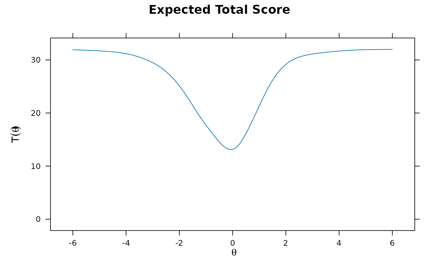plot(mod.combo, type = 'SE')

itemplot(mod.quad, 1, type = 'score')

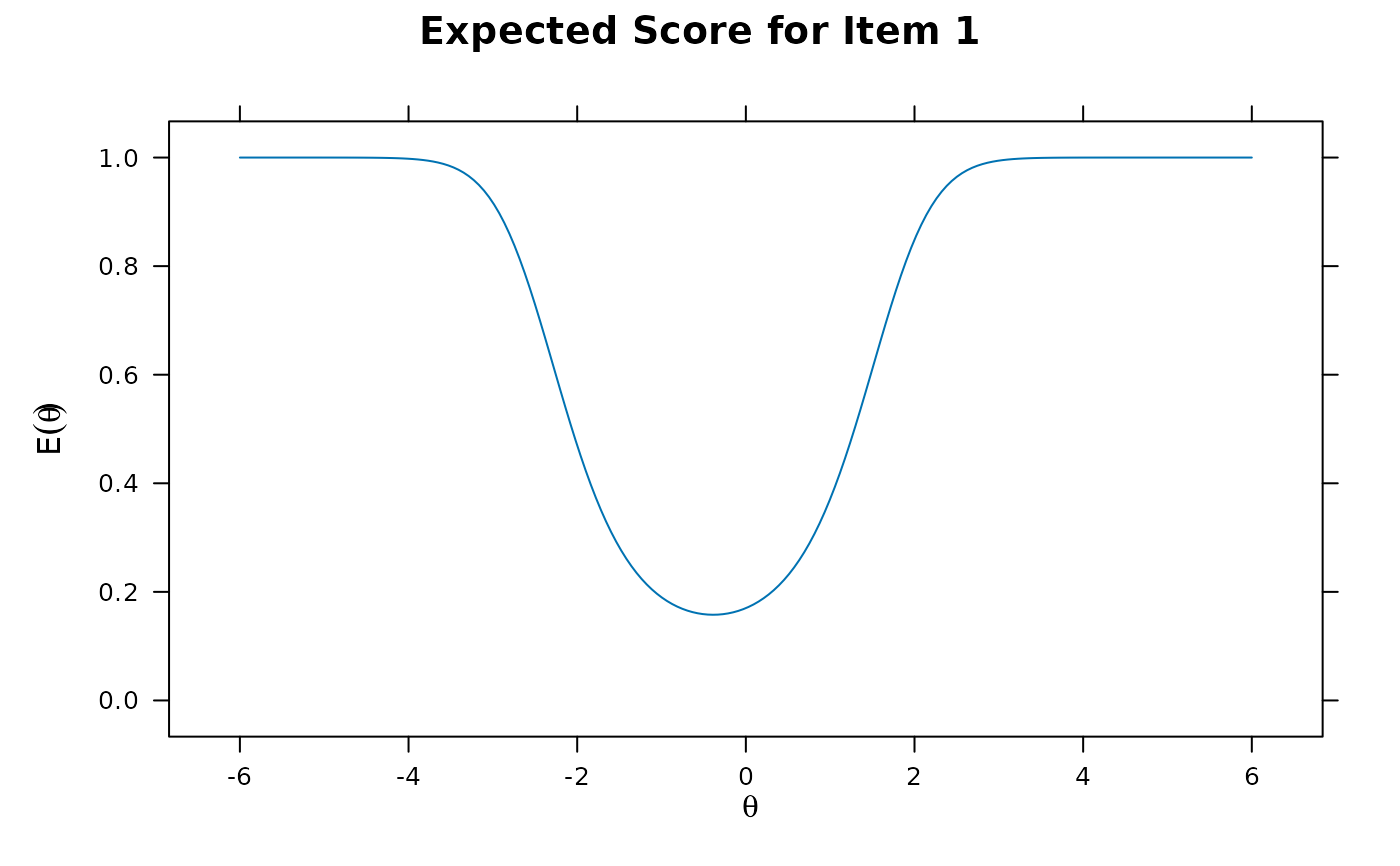itemplot(mod.combo, 2, type = 'score')

itemplot(mod.combo, 2, type = 'infocontour')


## empirical histogram examples (normal, skew and bimodality)
# make some data
set.seed(1234)
a <- matrix(rlnorm(50, .2, .2))
d <- matrix(rnorm(50))
ThetaNormal <- matrix(rnorm(2000))
ThetaBimodal <- scale(matrix(c(rnorm(1000, -2), rnorm(1000,2)))) #bimodal
ThetaSkew <- scale(matrix(rchisq(2000, 3))) #positive skew
datNormal <- simdata(a, d, 2000, itemtype = '2PL', Theta=ThetaNormal)
datBimodal <- simdata(a, d, 2000, itemtype = '2PL', Theta=ThetaBimodal)
datSkew <- simdata(a, d, 2000, itemtype = '2PL', Theta=ThetaSkew)

normal <- mirt(datNormal, 1, dentype = "empiricalhist")
#> 
plot(normal, type = 'empiricalhist')

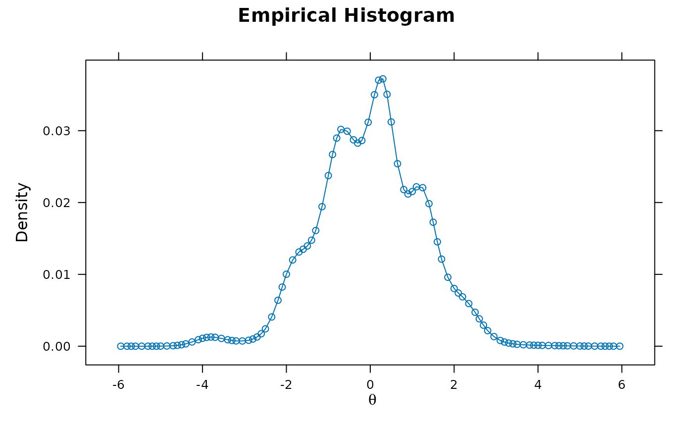histogram(ThetaNormal, breaks=30)


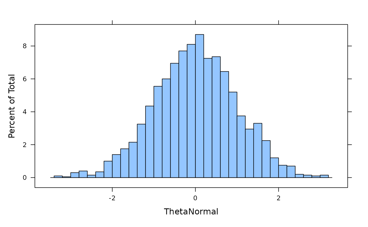bimodal <- mirt(datBimodal, 1, dentype = "empiricalhist")
#> 
plot(bimodal, type = 'empiricalhist')

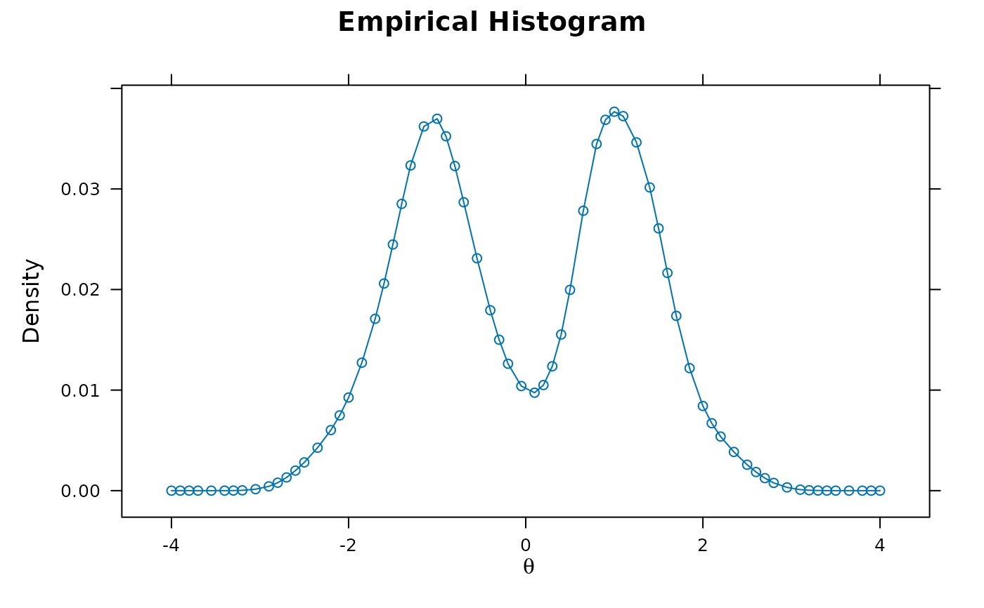histogram(ThetaBimodal, breaks=30)


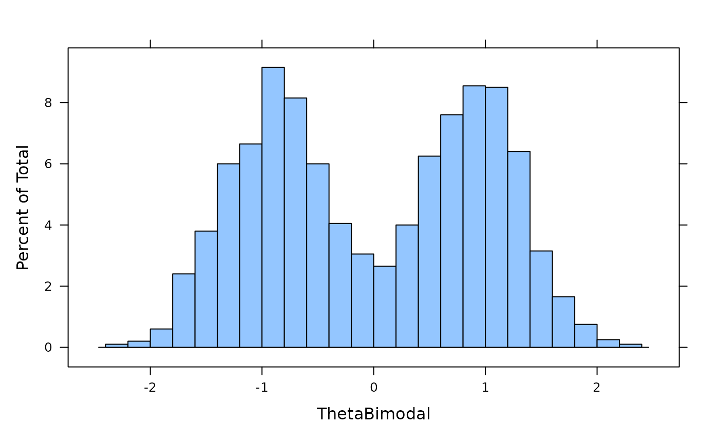skew <- mirt(datSkew, 1, dentype = "empiricalhist")
#> 
plot(skew, type = 'empiricalhist')

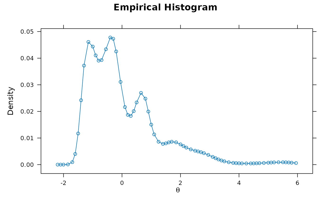histogram(ThetaSkew, breaks=30)


#####
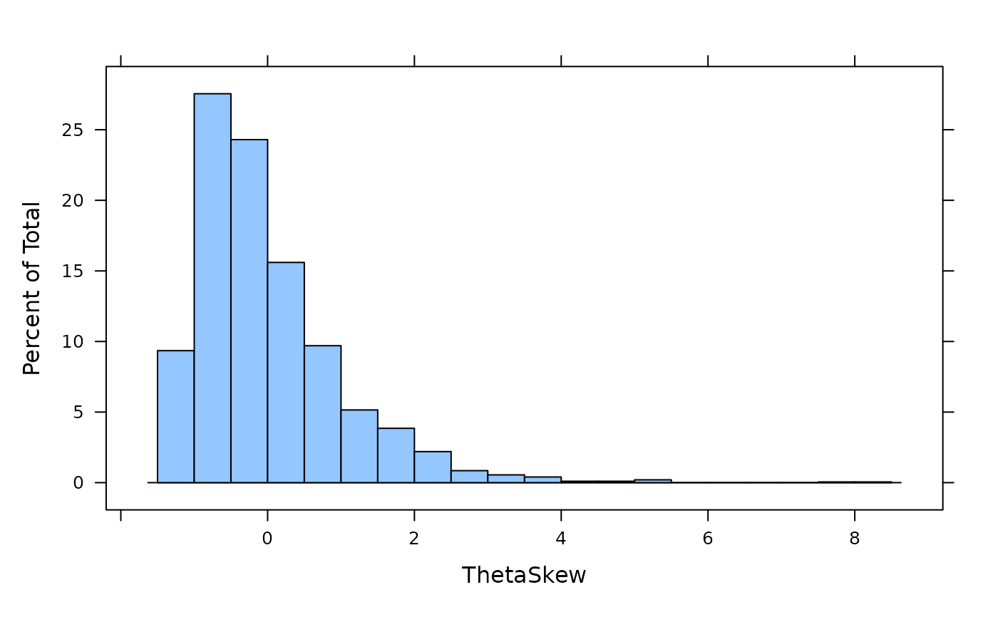# non-linear parameter constraints with Rsolnp package (nloptr supported as well):
# Find Rasch model subject to the constraint that the intercepts sum to 0

dat <- expand.table(LSAT6)
itemstats(dat)
#> $overall
#>     N mean_total.score sd_total.score ave.r sd.r alpha SEM.alpha
#>  1000            3.819          1.035 0.077 0.03 0.295     0.869
#> 
#> $itemstats
#>           N  mean    sd total.r total.r_if_rm alpha_if_rm
#> Item_1 1000 0.924 0.265   0.362         0.113       0.275
#> Item_2 1000 0.709 0.454   0.567         0.153       0.238
#> Item_3 1000 0.553 0.497   0.618         0.173       0.217
#> Item_4 1000 0.763 0.425   0.534         0.144       0.246
#> Item_5 1000 0.870 0.336   0.435         0.122       0.266
#> 
#> $proportions
#>            0     1
#> Item_1 0.076 0.924
#> Item_2 0.291 0.709
#> Item_3 0.447 0.553
#> Item_4 0.237 0.763
#> Item_5 0.130 0.870
#> 

# free latent mean and variance terms
model <- 'Theta = 1-5
          MEAN = Theta
          COV = Theta*Theta'

# view how vector of parameters is organized internally
sv <- mirt(dat, model, itemtype = 'Rasch', pars = 'values')
sv[sv$est, ]
#>    group   item     class   name parnum value lbound ubound  est const nconst
#> 2    all Item_1      dich      d      2 2.815   -Inf    Inf TRUE  none   none
#> 6    all Item_2      dich      d      6 1.082   -Inf    Inf TRUE  none   none
#> 10   all Item_3      dich      d     10 0.262   -Inf    Inf TRUE  none   none
#> 14   all Item_4      dich      d     14 1.407   -Inf    Inf TRUE  none   none
#> 18   all Item_5      dich      d     18 2.214   -Inf    Inf TRUE  none   none
#> 21   all  GROUP GroupPars MEAN_1     21 0.000   -Inf    Inf TRUE  none   none
#> 22   all  GROUP GroupPars COV_11     22 1.000      0    Inf TRUE  none   none
#>    prior.type prior_1 prior_2
#> 2        none     NaN     NaN
#> 6        none     NaN     NaN
#> 10       none     NaN     NaN
#> 14       none     NaN     NaN
#> 18       none     NaN     NaN
#> 21       none     NaN     NaN
#> 22       none     NaN     NaN

# constraint: create function for solnp to compute constraint, and declare value in eqB
eqfun <- function(p, optim_args) sum(p[1:5]) #could use browser() here, if it helps
LB <- c(rep(-15, 6), 1e-4) # more reasonable lower bound for variance term

mod <- mirt(dat, model, sv=sv, itemtype = 'Rasch', optimizer = 'solnp',
   solnp_args=list(eqfun=eqfun, eqB=0, LB=LB))
#> 
print(mod)
#> 
#> Call:
#> mirt(data = dat, model = model, itemtype = "Rasch", optimizer = "solnp", 
#>     solnp_args = list(eqfun = eqfun, eqB = 0, LB = LB), sv = sv)
#> 
#> Full-information item factor analysis with 1 factor(s).
#> Converged within 1e-04 tolerance after 34 EM iterations.
#> mirt version: 1.44.5 
#> M-step optimizer: solnp 
#> EM acceleration: Ramsay 
#> Number of rectangular quadrature: 61
#> Latent density type: Gaussian 
#> 
#> Log-likelihood = -2466.943
#> Estimated parameters: 7 
#> AIC = 4947.887
#> BIC = 4982.241; SABIC = 4960.009
#> G2 (25) = 21.81, p = 0.6467
#> RMSEA = 0, CFI = NaN, TLI = NaN
coef(mod)
#> $Item_1
#>     a1     d g u
#> par  1 1.253 0 1
#> 
#> $Item_2
#>     a1      d g u
#> par  1 -0.475 0 1
#> 
#> $Item_3
#>     a1      d g u
#> par  1 -1.233 0 1
#> 
#> $Item_4
#>     a1      d g u
#> par  1 -0.168 0 1
#> 
#> $Item_5
#>     a1     d g u
#> par  1 0.623 0 1
#> 
#> $GroupPars
#>     MEAN_1 COV_11
#> par  1.472  0.559
#> 
(ds <- sapply(coef(mod)[1:5], function(x) x[,'d']))
#>     Item_1     Item_2     Item_3     Item_4     Item_5 
#>  1.2529432 -0.4754429 -1.2327196 -0.1681687  0.6233879 
sum(ds)
#> [1] 4.635181e-15

# same likelihood location as: mirt(dat, 1, itemtype = 'Rasch')


#######
# latent regression Rasch model

# simulate data
set.seed(1234)
N <- 1000

# covariates
X1 <- rnorm(N); X2 <- rnorm(N)
covdata <- data.frame(X1, X2, X3 = rnorm(N))
Theta <- matrix(0.5 * X1 + -1 * X2 + rnorm(N, sd = 0.5))

# items and response data
a <- matrix(1, 20); d <- matrix(rnorm(20))
dat <- simdata(a, d, 1000, itemtype = '2PL', Theta=Theta)

# unconditional Rasch model
mod0 <- mirt(dat, 1, 'Rasch', SE=TRUE)
#> 
#> 
#> Calculating information matrix...
coef(mod0, printSE=TRUE)
#> $Item_1
#>     a1      d logit(g) logit(u)
#> par  1 -0.998     -999      999
#> SE  NA  0.085       NA       NA
#> 
#> $Item_2
#>     a1      d logit(g) logit(u)
#> par  1 -0.917     -999      999
#> SE  NA  0.085       NA       NA
#> 
#> $Item_3
#>     a1      d logit(g) logit(u)
#> par  1 -0.099     -999      999
#> SE  NA  0.081       NA       NA
#> 
#> $Item_4
#>     a1     d logit(g) logit(u)
#> par  1 1.893     -999      999
#> SE  NA 0.099       NA       NA
#> 
#> $Item_5
#>     a1     d logit(g) logit(u)
#> par  1 0.610     -999      999
#> SE  NA 0.082       NA       NA
#> 
#> $Item_6
#>     a1     d logit(g) logit(u)
#> par  1 1.071     -999      999
#> SE  NA 0.086       NA       NA
#> 
#> $Item_7
#>     a1      d logit(g) logit(u)
#> par  1 -0.074     -999      999
#> SE  NA  0.081       NA       NA
#> 
#> $Item_8
#>     a1      d logit(g) logit(u)
#> par  1 -1.405     -999      999
#> SE  NA  0.090       NA       NA
#> 
#> $Item_9
#>     a1     d logit(g) logit(u)
#> par  1 0.707     -999      999
#> SE  NA 0.083       NA       NA
#> 
#> $Item_10
#>     a1      d logit(g) logit(u)
#> par  1 -0.258     -999      999
#> SE  NA  0.081       NA       NA
#> 
#> $Item_11
#>     a1     d logit(g) logit(u)
#> par  1 0.336     -999      999
#> SE  NA 0.081       NA       NA
#> 
#> $Item_12
#>     a1     d logit(g) logit(u)
#> par  1 0.891     -999      999
#> SE  NA 0.084       NA       NA
#> 
#> $Item_13
#>     a1     d logit(g) logit(u)
#> par  1 0.653     -999      999
#> SE  NA 0.083       NA       NA
#> 
#> $Item_14
#>     a1      d logit(g) logit(u)
#> par  1 -1.942     -999      999
#> SE  NA  0.099       NA       NA
#> 
#> $Item_15
#>     a1      d logit(g) logit(u)
#> par  1 -2.143     -999      999
#> SE  NA  0.104       NA       NA
#> 
#> $Item_16
#>     a1     d logit(g) logit(u)
#> par  1 1.759     -999      999
#> SE  NA 0.096       NA       NA
#> 
#> $Item_17
#>     a1      d logit(g) logit(u)
#> par  1 -1.015     -999      999
#> SE  NA  0.085       NA       NA
#> 
#> $Item_18
#>     a1      d logit(g) logit(u)
#> par  1 -1.009     -999      999
#> SE  NA  0.085       NA       NA
#> 
#> $Item_19
#>     a1      d logit(g) logit(u)
#> par  1 -1.251     -999      999
#> SE  NA  0.088       NA       NA
#> 
#> $Item_20
#>     a1      d logit(g) logit(u)
#> par  1 -0.619     -999      999
#> SE  NA  0.082       NA       NA
#> 
#> $GroupPars
#>     MEAN_1 COV_11
#> par      0  1.393
#> SE      NA  0.085
#> 

# conditional model using X1, X2, and X3 (bad) as predictors of Theta
mod1 <- mirt(dat, 1, 'Rasch', covdata=covdata, formula = ~ X1 + X2 + X3, SE=TRUE)
#> 
#> 
#> Calculating information matrix...
coef(mod1, printSE=TRUE)
#> $Item_1
#>     a1      d logit(g) logit(u)
#> par  1 -0.967     -999      999
#> SE  NA  0.078       NA       NA
#> 
#> $Item_2
#>     a1      d logit(g) logit(u)
#> par  1 -0.887     -999      999
#> SE  NA  0.077       NA       NA
#> 
#> $Item_3
#>     a1      d logit(g) logit(u)
#> par  1 -0.068     -999      999
#> SE  NA  0.073       NA       NA
#> 
#> $Item_4
#>     a1     d logit(g) logit(u)
#> par  1 1.920     -999      999
#> SE  NA 0.092       NA       NA
#> 
#> $Item_5
#>     a1     d logit(g) logit(u)
#> par  1 0.640     -999      999
#> SE  NA 0.075       NA       NA
#> 
#> $Item_6
#>     a1     d logit(g) logit(u)
#> par  1 1.100     -999      999
#> SE  NA 0.079       NA       NA
#> 
#> $Item_7
#>     a1      d logit(g) logit(u)
#> par  1 -0.043     -999      999
#> SE  NA  0.073       NA       NA
#> 
#> $Item_8
#>     a1      d logit(g) logit(u)
#> par  1 -1.375     -999      999
#> SE  NA  0.083       NA       NA
#> 
#> $Item_9
#>     a1     d logit(g) logit(u)
#> par  1 0.737     -999      999
#> SE  NA 0.076       NA       NA
#> 
#> $Item_10
#>     a1      d logit(g) logit(u)
#> par  1 -0.227     -999      999
#> SE  NA  0.073       NA       NA
#> 
#> $Item_11
#>     a1     d logit(g) logit(u)
#> par  1 0.367     -999      999
#> SE  NA 0.074       NA       NA
#> 
#> $Item_12
#>     a1     d logit(g) logit(u)
#> par  1 0.921     -999      999
#> SE  NA 0.077       NA       NA
#> 
#> $Item_13
#>     a1     d logit(g) logit(u)
#> par  1 0.683     -999      999
#> SE  NA 0.075       NA       NA
#> 
#> $Item_14
#>     a1      d logit(g) logit(u)
#> par  1 -1.913     -999      999
#> SE  NA  0.093       NA       NA
#> 
#> $Item_15
#>     a1      d logit(g) logit(u)
#> par  1 -2.114     -999      999
#> SE  NA  0.098       NA       NA
#> 
#> $Item_16
#>     a1     d logit(g) logit(u)
#> par  1 1.786     -999      999
#> SE  NA 0.090       NA       NA
#> 
#> $Item_17
#>     a1      d logit(g) logit(u)
#> par  1 -0.985     -999      999
#> SE  NA  0.078       NA       NA
#> 
#> $Item_18
#>     a1      d logit(g) logit(u)
#> par  1 -0.979     -999      999
#> SE  NA  0.078       NA       NA
#> 
#> $Item_19
#>     a1      d logit(g) logit(u)
#> par  1 -1.221     -999      999
#> SE  NA  0.081       NA       NA
#> 
#> $Item_20
#>     a1      d logit(g) logit(u)
#> par  1 -0.589     -999      999
#> SE  NA  0.075       NA       NA
#> 
#> $GroupPars
#>     MEAN_1 COV_11
#> par      0  0.210
#> SE      NA  0.011
#> 
#> $lr.betas
#> $lr.betas$betas
#>                 F1
#> (Intercept)  0.000
#> X1           0.513
#> X2          -1.003
#> X3          -0.003
#> 
#> $lr.betas$SE
#>                F1
#> (Intercept)    NA
#> X1          0.015
#> X2          0.015
#> X3          0.014
#> 
#> 
coef(mod1, simplify=TRUE)
#> $items
#>         a1      d g u
#> Item_1   1 -0.967 0 1
#> Item_2   1 -0.887 0 1
#> Item_3   1 -0.068 0 1
#> Item_4   1  1.920 0 1
#> Item_5   1  0.640 0 1
#> Item_6   1  1.100 0 1
#> Item_7   1 -0.043 0 1
#> Item_8   1 -1.375 0 1
#> Item_9   1  0.737 0 1
#> Item_10  1 -0.227 0 1
#> Item_11  1  0.367 0 1
#> Item_12  1  0.921 0 1
#> Item_13  1  0.683 0 1
#> Item_14  1 -1.913 0 1
#> Item_15  1 -2.114 0 1
#> Item_16  1  1.786 0 1
#> Item_17  1 -0.985 0 1
#> Item_18  1 -0.979 0 1
#> Item_19  1 -1.221 0 1
#> Item_20  1 -0.589 0 1
#> 
#> $means
#> F1 
#>  0 
#> 
#> $cov
#>      F1
#> F1 0.21
#> 
#> $lr.betas
#> $lr.betas$betas
#>                 F1
#> (Intercept)  0.000
#> X1           0.513
#> X2          -1.003
#> X3          -0.003
#> 
#> $lr.betas$CI_2.5
#>                 F1
#> (Intercept)     NA
#> X1           0.485
#> X2          -1.032
#> X3          -0.031
#> 
#> $lr.betas$CI_97.5
#>                 F1
#> (Intercept)     NA
#> X1           0.542
#> X2          -0.974
#> X3           0.025
#> 
#> 
anova(mod0, mod1)  # jointly significant predictors of theta
#>           AIC    SABIC       HQ      BIC    logLik       X2 df p
#> mod0 21935.46 21971.83 21974.63 22038.53 -10946.73              
#> mod1 20756.61 20798.17 20801.38 20874.40 -10354.31 1184.851  3 0

# large sample z-ratios and p-values (if one cares)
cfs <- coef(mod1, printSE=TRUE)
(z <- cfs$lr.betas[[1]] / cfs$lr.betas[[2]])
#>                      F1
#> (Intercept)          NA
#> X1           35.2668946
#> X2          -67.5847949
#> X3           -0.2114561
round(pnorm(abs(z[,1]), lower.tail=FALSE)*2, 3)
#> (Intercept)          X1          X2          X3 
#>          NA       0.000       0.000       0.833 

# drop predictor for nested comparison
mod1b <- mirt(dat, 1, 'Rasch', covdata=covdata, formula = ~ X1 + X2)
#> 
anova(mod1b, mod1)
#>            AIC    SABIC       HQ      BIC    logLik    X2 df     p
#> mod1b 20754.63 20794.46 20797.53 20867.51 -10354.32               
#> mod1  20756.61 20798.17 20801.38 20874.40 -10354.31 0.018  1 0.893

# compare to mixedmirt() version of the same model
mod1.mixed <- mixedmirt(dat, 1, itemtype='Rasch',
                        covdata=covdata, lr.fixed = ~ X1 + X2 + X3, SE=TRUE)
#> , Max-Change = 0.1317, Max-Change = 0.1109, Max-Change = 0.0928, Max-Change = 0.2000, Max-Change = 0.0832, Max-Change = 0.0494, Max-Change = 0.0447, Max-Change = 0.0467, Max-Change = 0.0290, Max-Change = 0.0373, Max-Change = 0.0231, Max-Change = 0.0177, Max-Change = 0.0250, Max-Change = 0.0135, Max-Change = 0.0126, Max-Change = 0.0102, Max-Change = 0.0078, Max-Change = 0.0107, Max-Change = 0.0102, Max-Change = 0.0073, Max-Change = 0.0075, Max-Change = 0.0059, Max-Change = 0.0071, Max-Change = 0.0106, Max-Change = 0.0133, Max-Change = 0.0034, Max-Change = 0.0015, Max-Change = 0.0054, Max-Change = 0.0074, Max-Change = 0.0034, Max-Change = 0.0037, Max-Change = 0.0062, Max-Change = 0.0042, Max-Change = 0.0055, Max-Change = 0.0040, Max-Change = 0.0024, Max-Change = 0.0034, Max-Change = 0.0049, Max-Change = 0.0043, Max-Change = 0.0024, Max-Change = 0.0024, Max-Change = 0.0032, Max-Change = 0.0032, Max-Change = 0.0040, Max-Change = 0.0022, Max-Change = 0.0031, Max-Change = 0.0010, Max-Change = 0.0035, Max-Change = 0.0025, Max-Change = 0.0016, Max-Change = 0.0031, Max-Change = 0.0033, Max-Change = 0.0033, Max-Change = 0.0024, Max-Change = 0.0025, Max-Change = 0.0029, Max-Change = 0.0014, Max-Change = 0.0025, Max-Change = 0.0028, Max-Change = 0.0024, Max-Change = 0.0023, Max-Change = 0.0028, Max-Change = 0.0025, Max-Change = 0.0033, Max-Change = 0.0055, Max-Change = 0.0030, Max-Change = 0.0016, Max-Change = 0.0034, Max-Change = 0.0030, Max-Change = 0.0026, Max-Change = 0.0033, Max-Change = 0.0006, Max-Change = 0.0026, Max-Change = 0.0041, Max-Change = 0.0029, Max-Change = 0.0015, Max-Change = 0.0026, Max-Change = 0.0024, Max-Change = 0.0050, Max-Change = 0.0037, Max-Change = 0.0017, Max-Change = 0.0027, Max-Change = 0.0042, Max-Change = 0.0027, Max-Change = 0.0037, Max-Change = 0.0048, Max-Change = 0.0020, Max-Change = 0.0024, Max-Change = 0.0039, Max-Change = 0.0027, Max-Change = 0.0018, Max-Change = 0.0015, Max-Change = 0.0019, Max-Change = 0.0022, Max-Change = 0.0019, Max-Change = 0.0022, Max-Change = 0.0024, Max-Change = 0.0024, Max-Change = 0.0018, Max-Change = 0.0029, Max-Change = 0.0042, Max-Change = 0.0017, Max-Change = 0.0013, Max-Change = 0.0029, Max-Change = 0.0016, Max-Change = 0.0027, Max-Change = 0.0021, Max-Change = 0.0027, Max-Change = 0.0026, Max-Change = 0.0019, Max-Change = 0.0008, Max-Change = 0.0019, Max-Change = 0.0043, Max-Change = 0.0016, Max-Change = 0.0032, Max-Change = 0.0024, Max-Change = 0.0043, Max-Change = 0.0022, Max-Change = 0.0026, Max-Change = 0.0037, Max-Change = 0.0034, Max-Change = 0.0029, Max-Change = 0.0016, Max-Change = 0.0033, Max-Change = 0.0014, Max-Change = 0.0035, Max-Change = 0.0023, Max-Change = 0.0027, Max-Change = 0.0010, Max-Change = 0.0018, Max-Change = 0.0015, Max-Change = 0.0009, Max-Change = 0.0017, Max-Change = 0.0026, Max-Change = 0.0035, Max-Change = 0.0030, Max-Change = 0.0052, Max-Change = 0.0011, Max-Change = 0.0025, Max-Change = 0.0043, Max-Change = 0.0016, Max-Change = 0.0028, Max-Change = 0.0021, Max-Change = 0.0028, Max-Change = 0.0026, Max-Change = 0.0032, Max-Change = 0.0020, Max-Change = 0.0021, Max-Change = 0.0051, Max-Change = 0.0025, Max-Change = 0.0024, Max-Change = 0.0018, Max-Change = 0.0014, Max-Change = 0.0029, Max-Change = 0.0029, Max-Change = 0.0009, Max-Change = 0.0022, Max-Change = 0.0029, Max-Change = 0.0015, Max-Change = 0.0018, Max-Change = 0.0032, Max-Change = 0.0027, Max-Change = 0.0011, Max-Change = 0.0019, Max-Change = 0.0027, Max-Change = 0.0039, Max-Change = 0.0032, Max-Change = 0.0031, Max-Change = 0.0026, Max-Change = 0.0036, Max-Change = 0.0021, Max-Change = 0.0019, Max-Change = 0.0011, Max-Change = 0.0029, Max-Change = 0.0017, Max-Change = 0.0012, Max-Change = 0.0014, Max-Change = 0.0040, Max-Change = 0.0017, Max-Change = 0.0028, Max-Change = 0.0019, Max-Change = 0.0015, Max-Change = 0.0026, Max-Change = 0.0026, Max-Change = 0.0025, Max-Change = 0.0032, Max-Change = 0.0019, Max-Change = 0.0019, Max-Change = 0.0025, Max-Change = 0.0020, Max-Change = 0.0027, Max-Change = 0.0019, Max-Change = 0.0011, Max-Change = 0.0034, Max-Change = 0.0035, Max-Change = 0.0029, Max-Change = 0.0015, Max-Change = 0.0034, Max-Change = 0.0019, Max-Change = 0.0015, Max-Change = 0.0013, Max-Change = 0.0031, Max-Change = 0.0028, Max-Change = 0.0017, Max-Change = 0.0023, Max-Change = 0.0033, Max-Change = 0.0031, Max-Change = 0.0019, Max-Change = 0.0034, Max-Change = 0.0025, Max-Change = 0.0028, Max-Change = 0.0020, Max-Change = 0.0027, Max-Change = 0.0023, Max-Change = 0.0053, Max-Change = 0.0036, Max-Change = 0.0026, Max-Change = 0.0024, Max-Change = 0.0024, Max-Change = 0.0029, Max-Change = 0.0021, Max-Change = 0.0011, Max-Change = 0.0020, Max-Change = 0.0018, Max-Change = 0.0020, Max-Change = 0.0016, Max-Change = 0.0012, Max-Change = 0.0025, Max-Change = 0.0040, Max-Change = 0.0030, Max-Change = 0.0019, Max-Change = 0.0039, Max-Change = 0.0017, Max-Change = 0.0022, Max-Change = 0.0013, Max-Change = 0.0013, Max-Change = 0.0034, Max-Change = 0.0010, Max-Change = 0.0014, Max-Change = 0.0015, Max-Change = 0.0014, Max-Change = 0.0011, Max-Change = 0.0036, Max-Change = 0.0013, Max-Change = 0.0020, Max-Change = 0.0024, Max-Change = 0.0018, Max-Change = 0.0029, Max-Change = 0.0051, Max-Change = 0.0023, gam = 0.0000, Max-Change = 0.0000, gam = 0.1778, Max-Change = 0.0033, gam = 0.1057, Max-Change = 0.0012, gam = 0.0780, Max-Change = 0.0010, gam = 0.0629, Max-Change = 0.0005, gam = 0.0532, Max-Change = 0.0008, gam = 0.0464, Max-Change = 0.0006

#> 
#> Calculating information matrix...
#> 
#> Calculating log-likelihood...
coef(mod1.mixed)
#> $Item_1
#>         (Intercept) a1  d  g  u
#> par          -0.131  1  0  0  1
#> CI_2.5       -0.166 NA NA NA NA
#> CI_97.5      -0.097 NA NA NA NA
#> 
#> $Item_2
#>         (Intercept) a1  d  g  u
#> par          -0.131  1  0  0  1
#> CI_2.5       -0.166 NA NA NA NA
#> CI_97.5      -0.097 NA NA NA NA
#> 
#> $Item_3
#>         (Intercept) a1  d  g  u
#> par          -0.131  1  0  0  1
#> CI_2.5       -0.166 NA NA NA NA
#> CI_97.5      -0.097 NA NA NA NA
#> 
#> $Item_4
#>         (Intercept) a1  d  g  u
#> par          -0.131  1  0  0  1
#> CI_2.5       -0.166 NA NA NA NA
#> CI_97.5      -0.097 NA NA NA NA
#> 
#> $Item_5
#>         (Intercept) a1  d  g  u
#> par          -0.131  1  0  0  1
#> CI_2.5       -0.166 NA NA NA NA
#> CI_97.5      -0.097 NA NA NA NA
#> 
#> $Item_6
#>         (Intercept) a1  d  g  u
#> par          -0.131  1  0  0  1
#> CI_2.5       -0.166 NA NA NA NA
#> CI_97.5      -0.097 NA NA NA NA
#> 
#> $Item_7
#>         (Intercept) a1  d  g  u
#> par          -0.131  1  0  0  1
#> CI_2.5       -0.166 NA NA NA NA
#> CI_97.5      -0.097 NA NA NA NA
#> 
#> $Item_8
#>         (Intercept) a1  d  g  u
#> par          -0.131  1  0  0  1
#> CI_2.5       -0.166 NA NA NA NA
#> CI_97.5      -0.097 NA NA NA NA
#> 
#> $Item_9
#>         (Intercept) a1  d  g  u
#> par          -0.131  1  0  0  1
#> CI_2.5       -0.166 NA NA NA NA
#> CI_97.5      -0.097 NA NA NA NA
#> 
#> $Item_10
#>         (Intercept) a1  d  g  u
#> par          -0.131  1  0  0  1
#> CI_2.5       -0.166 NA NA NA NA
#> CI_97.5      -0.097 NA NA NA NA
#> 
#> $Item_11
#>         (Intercept) a1  d  g  u
#> par          -0.131  1  0  0  1
#> CI_2.5       -0.166 NA NA NA NA
#> CI_97.5      -0.097 NA NA NA NA
#> 
#> $Item_12
#>         (Intercept) a1  d  g  u
#> par          -0.131  1  0  0  1
#> CI_2.5       -0.166 NA NA NA NA
#> CI_97.5      -0.097 NA NA NA NA
#> 
#> $Item_13
#>         (Intercept) a1  d  g  u
#> par          -0.131  1  0  0  1
#> CI_2.5       -0.166 NA NA NA NA
#> CI_97.5      -0.097 NA NA NA NA
#> 
#> $Item_14
#>         (Intercept) a1  d  g  u
#> par          -0.131  1  0  0  1
#> CI_2.5       -0.166 NA NA NA NA
#> CI_97.5      -0.097 NA NA NA NA
#> 
#> $Item_15
#>         (Intercept) a1  d  g  u
#> par          -0.131  1  0  0  1
#> CI_2.5       -0.166 NA NA NA NA
#> CI_97.5      -0.097 NA NA NA NA
#> 
#> $Item_16
#>         (Intercept) a1  d  g  u
#> par          -0.131  1  0  0  1
#> CI_2.5       -0.166 NA NA NA NA
#> CI_97.5      -0.097 NA NA NA NA
#> 
#> $Item_17
#>         (Intercept) a1  d  g  u
#> par          -0.131  1  0  0  1
#> CI_2.5       -0.166 NA NA NA NA
#> CI_97.5      -0.097 NA NA NA NA
#> 
#> $Item_18
#>         (Intercept) a1  d  g  u
#> par          -0.131  1  0  0  1
#> CI_2.5       -0.166 NA NA NA NA
#> CI_97.5      -0.097 NA NA NA NA
#> 
#> $Item_19
#>         (Intercept) a1  d  g  u
#> par          -0.131  1  0  0  1
#> CI_2.5       -0.166 NA NA NA NA
#> CI_97.5      -0.097 NA NA NA NA
#> 
#> $Item_20
#>         (Intercept) a1  d  g  u
#> par          -0.131  1  0  0  1
#> CI_2.5       -0.166 NA NA NA NA
#> CI_97.5      -0.097 NA NA NA NA
#> 
#> $GroupPars
#>         MEAN_1 COV_11
#> par          0  0.087
#> CI_2.5      NA  0.068
#> CI_97.5     NA  0.105
#> 
#> $lr.betas
#>         F1_(Intercept) F1_X1  F1_X2  F1_X3
#> par                  0 0.409 -0.795 -0.007
#> CI_2.5              NA 0.376 -0.837 -0.040
#> CI_97.5             NA 0.441 -0.753  0.027
#> 
coef(mod1.mixed, printSE=TRUE)
#> $Item_1
#>     (Intercept) a1  d    g   u
#> par      -0.131  1  0 -999 999
#> SE        0.018 NA NA   NA  NA
#> 
#> $Item_2
#>     (Intercept) a1  d    g   u
#> par      -0.131  1  0 -999 999
#> SE        0.018 NA NA   NA  NA
#> 
#> $Item_3
#>     (Intercept) a1  d    g   u
#> par      -0.131  1  0 -999 999
#> SE        0.018 NA NA   NA  NA
#> 
#> $Item_4
#>     (Intercept) a1  d    g   u
#> par      -0.131  1  0 -999 999
#> SE        0.018 NA NA   NA  NA
#> 
#> $Item_5
#>     (Intercept) a1  d    g   u
#> par      -0.131  1  0 -999 999
#> SE        0.018 NA NA   NA  NA
#> 
#> $Item_6
#>     (Intercept) a1  d    g   u
#> par      -0.131  1  0 -999 999
#> SE        0.018 NA NA   NA  NA
#> 
#> $Item_7
#>     (Intercept) a1  d    g   u
#> par      -0.131  1  0 -999 999
#> SE        0.018 NA NA   NA  NA
#> 
#> $Item_8
#>     (Intercept) a1  d    g   u
#> par      -0.131  1  0 -999 999
#> SE        0.018 NA NA   NA  NA
#> 
#> $Item_9
#>     (Intercept) a1  d    g   u
#> par      -0.131  1  0 -999 999
#> SE        0.018 NA NA   NA  NA
#> 
#> $Item_10
#>     (Intercept) a1  d    g   u
#> par      -0.131  1  0 -999 999
#> SE        0.018 NA NA   NA  NA
#> 
#> $Item_11
#>     (Intercept) a1  d    g   u
#> par      -0.131  1  0 -999 999
#> SE        0.018 NA NA   NA  NA
#> 
#> $Item_12
#>     (Intercept) a1  d    g   u
#> par      -0.131  1  0 -999 999
#> SE        0.018 NA NA   NA  NA
#> 
#> $Item_13
#>     (Intercept) a1  d    g   u
#> par      -0.131  1  0 -999 999
#> SE        0.018 NA NA   NA  NA
#> 
#> $Item_14
#>     (Intercept) a1  d    g   u
#> par      -0.131  1  0 -999 999
#> SE        0.018 NA NA   NA  NA
#> 
#> $Item_15
#>     (Intercept) a1  d    g   u
#> par      -0.131  1  0 -999 999
#> SE        0.018 NA NA   NA  NA
#> 
#> $Item_16
#>     (Intercept) a1  d    g   u
#> par      -0.131  1  0 -999 999
#> SE        0.018 NA NA   NA  NA
#> 
#> $Item_17
#>     (Intercept) a1  d    g   u
#> par      -0.131  1  0 -999 999
#> SE        0.018 NA NA   NA  NA
#> 
#> $Item_18
#>     (Intercept) a1  d    g   u
#> par      -0.131  1  0 -999 999
#> SE        0.018 NA NA   NA  NA
#> 
#> $Item_19
#>     (Intercept) a1  d    g   u
#> par      -0.131  1  0 -999 999
#> SE        0.018 NA NA   NA  NA
#> 
#> $Item_20
#>     (Intercept) a1  d    g   u
#> par      -0.131  1  0 -999 999
#> SE        0.018 NA NA   NA  NA
#> 
#> $GroupPars
#>     MEAN_1 COV_11
#> par      0  0.087
#> SE      NA  0.009
#> 
#> $lr.betas
#>     F1_(Intercept) F1_X1  F1_X2  F1_X3
#> par              0 0.409 -0.795 -0.007
#> SE              NA 0.016  0.021  0.017
#> 

# draw plausible values for secondary analyses
pv <- fscores(mod1, plausible.draws = 10)
pvmods <- lapply(pv, function(x, covdata) lm(x ~ covdata$X1 + covdata$X2),
                 covdata=covdata)
# population characteristics recovered well, and can be averaged over
so <- lapply(pvmods, summary)
so
#> [[1]]
#> 
#> Call:
#> lm(formula = x ~ covdata$X1 + covdata$X2)
#> 
#> Residuals:
#>      Min       1Q   Median       3Q      Max 
#> -1.26648 -0.32520 -0.01075  0.33305  1.62905 
#> 
#> Coefficients:
#>             Estimate Std. Error t value Pr(>|t|)    
#> (Intercept) -0.01238    0.01486  -0.833    0.405    
#> covdata$X1   0.52045    0.01492  34.875   <2e-16 ***
#> covdata$X2  -1.00015    0.01517 -65.934   <2e-16 ***
#> ---
#> Signif. codes:  0 ‘***’ 0.001 ‘**’ 0.01 ‘*’ 0.05 ‘.’ 0.1 ‘ ’ 1
#> 
#> Residual standard error: 0.4697 on 997 degrees of freedom
#> Multiple R-squared:  0.8422,	Adjusted R-squared:  0.8419 
#> F-statistic:  2660 on 2 and 997 DF,  p-value: < 2.2e-16
#> 
#> 
#> [[2]]
#> 
#> Call:
#> lm(formula = x ~ covdata$X1 + covdata$X2)
#> 
#> Residuals:
#>      Min       1Q   Median       3Q      Max 
#> -1.32562 -0.28616 -0.00154  0.28891  1.39971 
#> 
#> Coefficients:
#>             Estimate Std. Error t value Pr(>|t|)    
#> (Intercept) -0.01017    0.01429  -0.712    0.477    
#> covdata$X1   0.50739    0.01435  35.351   <2e-16 ***
#> covdata$X2  -1.00565    0.01459 -68.931   <2e-16 ***
#> ---
#> Signif. codes:  0 ‘***’ 0.001 ‘**’ 0.01 ‘*’ 0.05 ‘.’ 0.1 ‘ ’ 1
#> 
#> Residual standard error: 0.4517 on 997 degrees of freedom
#> Multiple R-squared:  0.8521,	Adjusted R-squared:  0.8518 
#> F-statistic:  2872 on 2 and 997 DF,  p-value: < 2.2e-16
#> 
#> 
#> [[3]]
#> 
#> Call:
#> lm(formula = x ~ covdata$X1 + covdata$X2)
#> 
#> Residuals:
#>      Min       1Q   Median       3Q      Max 
#> -1.35140 -0.31731 -0.02494  0.31557  1.37706 
#> 
#> Coefficients:
#>              Estimate Std. Error t value Pr(>|t|)    
#> (Intercept)  0.001808   0.014577   0.124    0.901    
#> covdata$X1   0.509447   0.014639  34.800   <2e-16 ***
#> covdata$X2  -0.996418   0.014880 -66.963   <2e-16 ***
#> ---
#> Signif. codes:  0 ‘***’ 0.001 ‘**’ 0.01 ‘*’ 0.05 ‘.’ 0.1 ‘ ’ 1
#> 
#> Residual standard error: 0.4607 on 997 degrees of freedom
#> Multiple R-squared:  0.8453,	Adjusted R-squared:  0.845 
#> F-statistic:  2724 on 2 and 997 DF,  p-value: < 2.2e-16
#> 
#> 
#> [[4]]
#> 
#> Call:
#> lm(formula = x ~ covdata$X1 + covdata$X2)
#> 
#> Residuals:
#>      Min       1Q   Median       3Q      Max 
#> -1.32336 -0.31714  0.00293  0.30301  1.52789 
#> 
#> Coefficients:
#>             Estimate Std. Error t value Pr(>|t|)    
#> (Intercept)  0.01217    0.01436   0.848    0.397    
#> covdata$X1   0.51991    0.01442  36.046   <2e-16 ***
#> covdata$X2  -1.00457    0.01466 -68.521   <2e-16 ***
#> ---
#> Signif. codes:  0 ‘***’ 0.001 ‘**’ 0.01 ‘*’ 0.05 ‘.’ 0.1 ‘ ’ 1
#> 
#> Residual standard error: 0.4539 on 997 degrees of freedom
#> Multiple R-squared:  0.8519,	Adjusted R-squared:  0.8516 
#> F-statistic:  2867 on 2 and 997 DF,  p-value: < 2.2e-16
#> 
#> 
#> [[5]]
#> 
#> Call:
#> lm(formula = x ~ covdata$X1 + covdata$X2)
#> 
#> Residuals:
#>      Min       1Q   Median       3Q      Max 
#> -1.57068 -0.30988  0.01011  0.32299  1.65455 
#> 
#> Coefficients:
#>             Estimate Std. Error t value Pr(>|t|)    
#> (Intercept)  0.01728    0.01451   1.191    0.234    
#> covdata$X1   0.51845    0.01458  35.570   <2e-16 ***
#> covdata$X2  -1.02688    0.01482 -69.313   <2e-16 ***
#> ---
#> Signif. codes:  0 ‘***’ 0.001 ‘**’ 0.01 ‘*’ 0.05 ‘.’ 0.1 ‘ ’ 1
#> 
#> Residual standard error: 0.4587 on 997 degrees of freedom
#> Multiple R-squared:  0.8535,	Adjusted R-squared:  0.8532 
#> F-statistic:  2904 on 2 and 997 DF,  p-value: < 2.2e-16
#> 
#> 
#> [[6]]
#> 
#> Call:
#> lm(formula = x ~ covdata$X1 + covdata$X2)
#> 
#> Residuals:
#>      Min       1Q   Median       3Q      Max 
#> -1.62908 -0.33205  0.01795  0.30914  1.30377 
#> 
#> Coefficients:
#>              Estimate Std. Error t value Pr(>|t|)    
#> (Intercept)  0.002797   0.014490   0.193    0.847    
#> covdata$X1   0.532558   0.014553  36.595   <2e-16 ***
#> covdata$X2  -0.993287   0.014792 -67.150   <2e-16 ***
#> ---
#> Signif. codes:  0 ‘***’ 0.001 ‘**’ 0.01 ‘*’ 0.05 ‘.’ 0.1 ‘ ’ 1
#> 
#> Residual standard error: 0.458 on 997 degrees of freedom
#> Multiple R-squared:  0.8486,	Adjusted R-squared:  0.8483 
#> F-statistic:  2794 on 2 and 997 DF,  p-value: < 2.2e-16
#> 
#> 
#> [[7]]
#> 
#> Call:
#> lm(formula = x ~ covdata$X1 + covdata$X2)
#> 
#> Residuals:
#>      Min       1Q   Median       3Q      Max 
#> -1.34299 -0.29638  0.00163  0.29823  1.38556 
#> 
#> Coefficients:
#>             Estimate Std. Error t value Pr(>|t|)    
#> (Intercept) -0.01742    0.01431  -1.218    0.224    
#> covdata$X1   0.51034    0.01437  35.515   <2e-16 ***
#> covdata$X2  -0.98395    0.01461 -67.365   <2e-16 ***
#> ---
#> Signif. codes:  0 ‘***’ 0.001 ‘**’ 0.01 ‘*’ 0.05 ‘.’ 0.1 ‘ ’ 1
#> 
#> Residual standard error: 0.4522 on 997 degrees of freedom
#> Multiple R-squared:  0.8476,	Adjusted R-squared:  0.8473 
#> F-statistic:  2773 on 2 and 997 DF,  p-value: < 2.2e-16
#> 
#> 
#> [[8]]
#> 
#> Call:
#> lm(formula = x ~ covdata$X1 + covdata$X2)
#> 
#> Residuals:
#>      Min       1Q   Median       3Q      Max 
#> -1.58071 -0.29398 -0.00239  0.30383  1.50535 
#> 
#> Coefficients:
#>              Estimate Std. Error t value Pr(>|t|)    
#> (Intercept)  0.001433   0.014413   0.099    0.921    
#> covdata$X1   0.505478   0.014475  34.920   <2e-16 ***
#> covdata$X2  -1.036824   0.014714 -70.467   <2e-16 ***
#> ---
#> Signif. codes:  0 ‘***’ 0.001 ‘**’ 0.01 ‘*’ 0.05 ‘.’ 0.1 ‘ ’ 1
#> 
#> Residual standard error: 0.4556 on 997 degrees of freedom
#> Multiple R-squared:  0.856,	Adjusted R-squared:  0.8557 
#> F-statistic:  2963 on 2 and 997 DF,  p-value: < 2.2e-16
#> 
#> 
#> [[9]]
#> 
#> Call:
#> lm(formula = x ~ covdata$X1 + covdata$X2)
#> 
#> Residuals:
#>      Min       1Q   Median       3Q      Max 
#> -1.54224 -0.30795 -0.01978  0.30469  1.55104 
#> 
#> Coefficients:
#>             Estimate Std. Error t value Pr(>|t|)    
#> (Intercept) -0.01015    0.01421  -0.714    0.475    
#> covdata$X1   0.48654    0.01428  34.081   <2e-16 ***
#> covdata$X2  -0.98823    0.01451 -68.103   <2e-16 ***
#> ---
#> Signif. codes:  0 ‘***’ 0.001 ‘**’ 0.01 ‘*’ 0.05 ‘.’ 0.1 ‘ ’ 1
#> 
#> Residual standard error: 0.4493 on 997 degrees of freedom
#> Multiple R-squared:  0.8478,	Adjusted R-squared:  0.8475 
#> F-statistic:  2777 on 2 and 997 DF,  p-value: < 2.2e-16
#> 
#> 
#> [[10]]
#> 
#> Call:
#> lm(formula = x ~ covdata$X1 + covdata$X2)
#> 
#> Residuals:
#>      Min       1Q   Median       3Q      Max 
#> -1.58687 -0.30844 -0.01915  0.30946  1.64039 
#> 
#> Coefficients:
#>              Estimate Std. Error t value Pr(>|t|)    
#> (Intercept) -0.003936   0.014763  -0.267     0.79    
#> covdata$X1   0.487032   0.014826  32.850   <2e-16 ***
#> covdata$X2  -1.014430   0.015070 -67.315   <2e-16 ***
#> ---
#> Signif. codes:  0 ‘***’ 0.001 ‘**’ 0.01 ‘*’ 0.05 ‘.’ 0.1 ‘ ’ 1
#> 
#> Residual standard error: 0.4666 on 997 degrees of freedom
#> Multiple R-squared:  0.8436,	Adjusted R-squared:  0.8433 
#> F-statistic:  2689 on 2 and 997 DF,  p-value: < 2.2e-16
#> 
#> 

# compute Rubin's multiple imputation average
par <- lapply(so, function(x) x$coefficients[, 'Estimate'])
SEpar <- lapply(so, function(x) x$coefficients[, 'Std. Error'])
averageMI(par, SEpar)
#>                par SEpar       t     df    p
#> (Intercept) -0.002 0.019  -0.100 58.701 0.23
#> covdata$X1   0.510 0.021  24.225 32.982    0
#> covdata$X2  -1.005 0.023 -43.701 26.131    0

############
# Example using Gauss-Hermite quadrature with custom input functions

if (FALSE) { # \dontrun{
library(fastGHQuad)
data(SAT12)
data <- key2binary(SAT12,
                   key = c(1,4,5,2,3,1,2,1,3,1,2,4,2,1,5,3,4,4,1,4,3,3,4,1,3,5,1,3,1,5,4,5))
GH <- gaussHermiteData(50)
Theta <- matrix(GH$x)

# This prior works for uni- and multi-dimensional models
prior <- function(Theta, Etable){
    P <- grid <- GH$w / sqrt(pi)
    if(ncol(Theta) > 1)
        for(i in 2:ncol(Theta))
            P <- expand.grid(P, grid)
     if(!is.vector(P)) P <- apply(P, 1, prod)
     P
}

GHmod1 <- mirt(data, 1, optimizer = 'NR',
              technical = list(customTheta = Theta, customPriorFun = prior))
coef(GHmod1, simplify=TRUE)

Theta2 <- as.matrix(expand.grid(Theta, Theta))
GHmod2 <- mirt(data, 2, optimizer = 'NR', TOL = .0002,
              technical = list(customTheta = Theta2, customPriorFun = prior))
summary(GHmod2, suppress=.2)
} # }

############
# Davidian curve example

dat <- key2binary(SAT12,
                   key = c(1,4,5,2,3,1,2,1,3,1,2,4,2,1,5,3,4,4,1,4,3,3,4,1,3,5,1,3,1,5,4,5))
dav <- mirt(dat, 1, dentype = 'Davidian-4') # use four smoothing parameters
#> 
plot(dav, type = 'Davidian') # shape of latent trait distribution

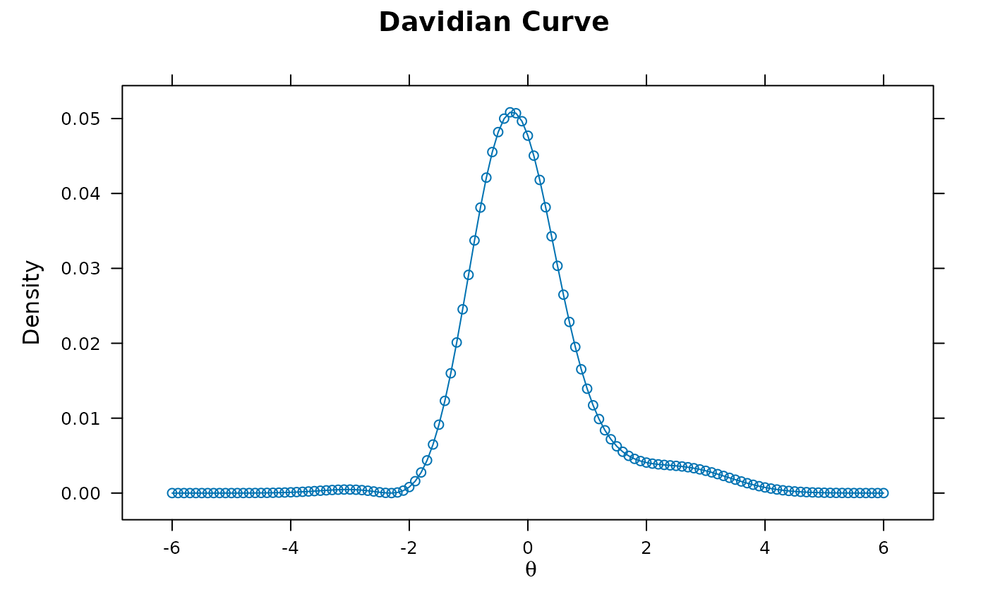coef(dav, simplify=TRUE)
#> $items
#>            a1      d g u
#> Item.1  0.774 -1.048 0 1
#> Item.2  1.684  0.495 0 1
#> Item.3  1.051 -1.114 0 1
#> Item.4  0.582 -0.531 0 1
#> Item.5  1.043  0.613 0 1
#> Item.6  1.037 -2.030 0 1
#> Item.7  1.096  1.397 0 1
#> Item.8  0.639 -1.513 0 1
#> Item.9  0.543  2.128 0 1
#> Item.10 0.993 -0.352 0 1
#> Item.11 2.130  5.453 0 1
#> Item.12 0.163 -0.338 0 1
#> Item.13 1.204  0.867 0 1
#> Item.14 1.171  1.211 0 1
#> Item.15 1.387  1.925 0 1
#> Item.16 0.725 -0.389 0 1
#> Item.17 1.860  4.273 0 1
#> Item.18 1.763 -0.788 0 1
#> Item.19 0.880  0.236 0 1
#> Item.20 1.866  2.743 0 1
#> Item.21 0.695  2.552 0 1
#> Item.22 1.863  3.592 0 1
#> Item.23 0.590 -0.851 0 1
#> Item.24 1.335  1.296 0 1
#> Item.25 0.733 -0.558 0 1
#> Item.26 1.649 -0.125 0 1
#> Item.27 2.356  2.968 0 1
#> Item.28 1.060  0.184 0 1
#> Item.29 0.803 -0.742 0 1
#> Item.30 0.352 -0.241 0 1
#> Item.31 2.944  3.061 0 1
#> Item.32 0.169 -1.651 0 1
#> 
#> $means
#> F1 
#>  0 
#> 
#> $cov
#>    F1
#> F1  1
#> 
#> $Davidian_phis
#> [1]  1.289  0.086 -0.443  1.245
#> 

fs <- fscores(dav) # assume normal prior
fs2 <- fscores(dav, use_dentype_estimate=TRUE) # use Davidian estimated prior shape
head(cbind(fs, fs2))
#>               F1           F1
#> [1,]  2.66818540  3.599616034
#> [2,]  0.14648879  0.070501775
#> [3,]  0.06802365  0.004037417
#> [4,] -0.41577386 -0.426755059
#> [5,]  0.67027700  0.559830142
#> [6,]  0.45477422  0.353831282

itemfit(dav) # assume normal prior
#> Error: Only X2, G2, PV_Q1, PV_Q1*, infit, X2*, and X2*_df can be computed with missing data.
#>              Pass na.rm=TRUE to remove missing data row-wise
itemfit(dav, use_dentype_estimate=TRUE) # use Davidian estimated prior shape
#> Error: Only X2, G2, PV_Q1, PV_Q1*, infit, X2*, and X2*_df can be computed with missing data.
#>              Pass na.rm=TRUE to remove missing data row-wise

############
# Unfolding models

# polytomous hyperbolic cosine model with
#  estimated latitude of acceptance (rho parameters)
mod <- mirt(Science, model=1, itemtype = 'hcm')
#> 
coef(mod, simplify=TRUE)$items
#>         a1        d log_rho1 log_rho2  log_rho3
#> Comfort  1 1.989655 1.625421 1.526102 -16.17198
#> Work     1 2.485054 1.478531 1.224489 -20.39161
#> Future   1 1.801569 1.491945 1.185052 -15.30324
#> Benefit  1 1.903674 1.471276 1.039336 -17.53716
coef(mod, simplify=TRUE, IRTpars=TRUE)$items
#>         a         b     rho1     rho2         rho3
#> Comfort 1 -1.989655 5.080557 4.600212 9.475379e-08
#> Work    1 -2.485054 4.386497 3.402426 1.393270e-09
#> Future  1 -1.801569 4.445732 3.270856 2.258856e-07
#> Benefit 1 -1.903674 4.354789 2.827339 2.419408e-08

plot(mod)

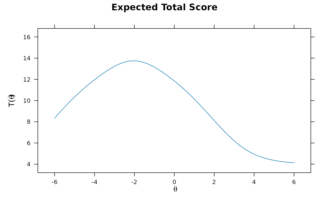plot(mod, type = 'trace')

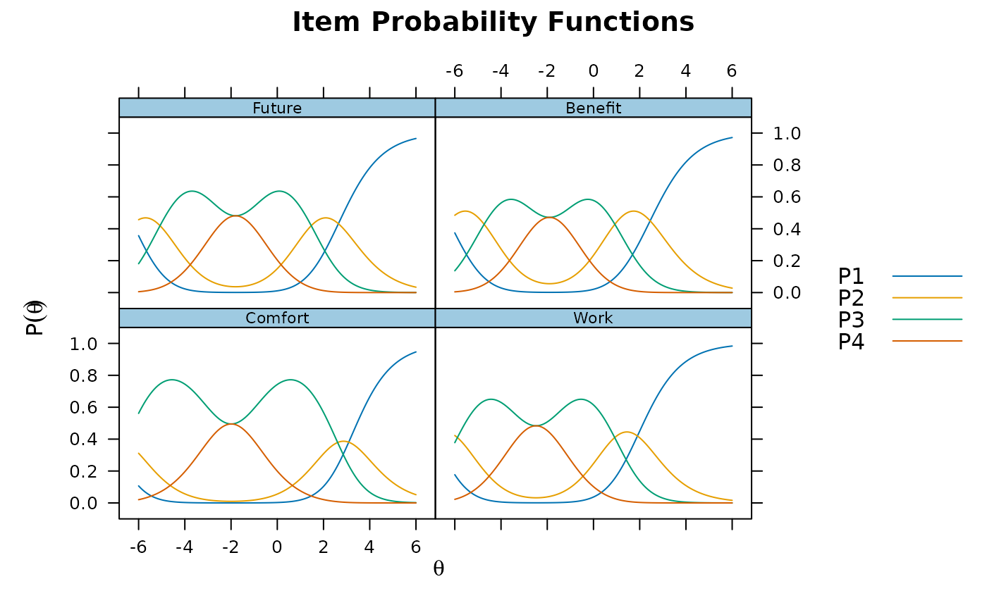plot(mod, type = 'itemscore')


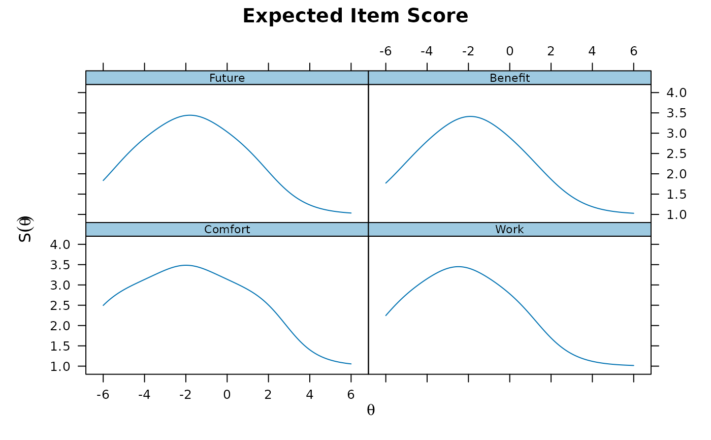# EAP estimates
fs <- fscores(mod)
head(fs)
#>              F1
#> [1,] -0.6675994
#> [2,] -0.1584800
#> [3,]  0.6560938
#> [4,]  0.6560938
#> [5,] -0.2058628
#> [6,] -1.0079077

itemfit(mod)
#>      item   S_X2 df.S_X2 RMSEA.S_X2 p.S_X2
#> 1 Comfort  4.437       6      0.000  0.618
#> 2    Work 10.778       8      0.030  0.215
#> 3  Future 18.242      10      0.046  0.051
#> 4 Benefit 12.020      11      0.015  0.362
M2(mod, type = 'C2')
#>             M2 df            p     RMSEA    RMSEA_5 RMSEA_95      TLI       CFI
#> stats 18.78276  2 8.344004e-05 0.1464969 0.09063855 0.209979 0.736325 0.9121083

###########
# 5PL and restricted 5PL example
dat <- expand.table(LSAT7)

mod2PL <- mirt(dat)
#> 
mod2PL
#> 
#> Call:
#> mirt(data = dat)
#> 
#> Full-information item factor analysis with 1 factor(s).
#> Converged within 1e-04 tolerance after 28 EM iterations.
#> mirt version: 1.44.5 
#> M-step optimizer: BFGS 
#> EM acceleration: Ramsay 
#> Number of rectangular quadrature: 61
#> Latent density type: Gaussian 
#> 
#> Log-likelihood = -2658.805
#> Estimated parameters: 10 
#> AIC = 5337.61
#> BIC = 5386.688; SABIC = 5354.927
#> G2 (21) = 31.7, p = 0.0628
#> RMSEA = 0.023, CFI = NaN, TLI = NaN

# Following does not converge without including strong priors
# mod5PL <- mirt(dat, itemtype = '5PL')
# mod5PL

# restricted version of 5PL (asymmetric 2PL)
model <- 'Theta = 1-5
          FIXED = (1-5, g), (1-5, u)'

mod2PL_asym <- mirt(dat, model=model, itemtype = '5PL')
#> 
mod2PL_asym
#> 
#> Call:
#> mirt(data = dat, model = model, itemtype = "5PL")
#> 
#> Full-information item factor analysis with 1 factor(s).
#> Converged within 1e-04 tolerance after 69 EM iterations.
#> mirt version: 1.44.5 
#> M-step optimizer: BFGS 
#> EM acceleration: Ramsay 
#> Number of rectangular quadrature: 61
#> Latent density type: Gaussian 
#> 
#> Log-likelihood = -2657.911
#> Estimated parameters: 15 
#> AIC = 5345.822
#> BIC = 5419.438; SABIC = 5371.797
#> G2 (16) = 29.91, p = 0.0185
#> RMSEA = 0.03, CFI = NaN, TLI = NaN
coef(mod2PL_asym, simplify=TRUE)
#> $items
#>           a1      d g u   logS
#> Item.1 0.926  2.882 0 1  0.962
#> Item.2 2.141 -1.547 0 1 -1.454
#> Item.3 1.589  2.066 0 1  0.264
#> Item.4 0.613  2.223 0 1  1.518
#> Item.5 0.748  1.948 0 1  0.079
#> 
#> $means
#> Theta 
#>     0 
#> 
#> $cov
#>       Theta
#> Theta     1
#> 
coef(mod2PL_asym, simplify=TRUE, IRTpars=TRUE)
#> $items
#>            a      b g u     S
#> Item.1 0.926 -3.113 0 1 2.618
#> Item.2 2.141  0.722 0 1 0.234
#> Item.3 1.589 -1.301 0 1 1.301
#> Item.4 0.613 -3.627 0 1 4.563
#> Item.5 0.748 -2.605 0 1 1.082
#> 
#> $means
#> Theta 
#>     0 
#> 
#> $cov
#>       Theta
#> Theta     1
#> 

# no big difference statistically or visually
anova(mod2PL, mod2PL_asym)
#>                  AIC    SABIC       HQ      BIC    logLik    X2 df     p
#> mod2PL      5337.610 5354.927 5356.263 5386.688 -2658.805               
#> mod2PL_asym 5345.822 5371.797 5373.801 5419.438 -2657.911 1.788  5 0.878
plot(mod2PL, type = 'trace')

plot(mod2PL_asym, type = 'trace')



###################
# LLTM example

a <- matrix(rep(1,30))
d <- rep(c(1,0, -1),each = 10)  # first easy, then medium, last difficult
dat <- simdata(a, d, 1000, itemtype = '2PL')

# unconditional model for intercept comparisons
mod <- mirt(dat, itemtype = 'Rasch')
#> 
coef(mod, simplify=TRUE)
#> $items
#>         a1      d g u
#> Item_1   1  0.865 0 1
#> Item_2   1  0.969 0 1
#> Item_3   1  1.002 0 1
#> Item_4   1  1.053 0 1
#> Item_5   1  1.002 0 1
#> Item_6   1  1.013 0 1
#> Item_7   1  1.030 0 1
#> Item_8   1  1.013 0 1
#> Item_9   1  1.024 0 1
#> Item_10  1  0.914 0 1
#> Item_11  1  0.038 0 1
#> Item_12  1 -0.044 0 1
#> Item_13  1 -0.092 0 1
#> Item_14  1  0.014 0 1
#> Item_15  1  0.048 0 1
#> Item_16  1  0.033 0 1
#> Item_17  1 -0.063 0 1
#> Item_18  1  0.000 0 1
#> Item_19  1  0.004 0 1
#> Item_20  1 -0.101 0 1
#> Item_21  1 -1.013 0 1
#> Item_22  1 -1.013 0 1
#> Item_23  1 -1.053 0 1
#> Item_24  1 -0.985 0 1
#> Item_25  1 -0.996 0 1
#> Item_26  1 -0.985 0 1
#> Item_27  1 -0.924 0 1
#> Item_28  1 -0.870 0 1
#> Item_29  1 -0.848 0 1
#> Item_30  1 -0.935 0 1
#> 
#> $means
#> F1 
#>  0 
#> 
#> $cov
#>       F1
#> F1 0.949
#> 

# Suppose that the first 10 items were suspected to be easy, followed by 10 medium difficulty items,
# then finally the last 10 items are difficult,
# and we wish to test this item structure hypothesis (more intercept designs are possible
# by including more columns).
itemdesign <- data.frame(difficulty =
   factor(c(rep('easy', 10), rep('medium', 10), rep('hard', 10))))
rownames(itemdesign) <- colnames(dat)
itemdesign
#>         difficulty
#> Item_1        easy
#> Item_2        easy
#> Item_3        easy
#> Item_4        easy
#> Item_5        easy
#> Item_6        easy
#> Item_7        easy
#> Item_8        easy
#> Item_9        easy
#> Item_10       easy
#> Item_11     medium
#> Item_12     medium
#> Item_13     medium
#> Item_14     medium
#> Item_15     medium
#> Item_16     medium
#> Item_17     medium
#> Item_18     medium
#> Item_19     medium
#> Item_20     medium
#> Item_21       hard
#> Item_22       hard
#> Item_23       hard
#> Item_24       hard
#> Item_25       hard
#> Item_26       hard
#> Item_27       hard
#> Item_28       hard
#> Item_29       hard
#> Item_30       hard

# LLTM with mirt()
lltm <- mirt(dat, itemtype = 'Rasch', SE=TRUE,
   item.formula = ~ 0 + difficulty, itemdesign=itemdesign)
#> 
#> 
#> Calculating information matrix...
coef(lltm, simplify=TRUE)
#> $items
#>         difficultyeasy difficultyhard difficultymedium a1 d g u
#> Item_1           0.988          0.000            0.000  1 0 0 1
#> Item_2           0.988          0.000            0.000  1 0 0 1
#> Item_3           0.988          0.000            0.000  1 0 0 1
#> Item_4           0.988          0.000            0.000  1 0 0 1
#> Item_5           0.988          0.000            0.000  1 0 0 1
#> Item_6           0.988          0.000            0.000  1 0 0 1
#> Item_7           0.988          0.000            0.000  1 0 0 1
#> Item_8           0.988          0.000            0.000  1 0 0 1
#> Item_9           0.988          0.000            0.000  1 0 0 1
#> Item_10          0.988          0.000            0.000  1 0 0 1
#> Item_11          0.000          0.000           -0.017  1 0 0 1
#> Item_12          0.000          0.000           -0.017  1 0 0 1
#> Item_13          0.000          0.000           -0.017  1 0 0 1
#> Item_14          0.000          0.000           -0.017  1 0 0 1
#> Item_15          0.000          0.000           -0.017  1 0 0 1
#> Item_16          0.000          0.000           -0.017  1 0 0 1
#> Item_17          0.000          0.000           -0.017  1 0 0 1
#> Item_18          0.000          0.000           -0.017  1 0 0 1
#> Item_19          0.000          0.000           -0.017  1 0 0 1
#> Item_20          0.000          0.000           -0.017  1 0 0 1
#> Item_21          0.000         -0.962            0.000  1 0 0 1
#> Item_22          0.000         -0.962            0.000  1 0 0 1
#> Item_23          0.000         -0.962            0.000  1 0 0 1
#> Item_24          0.000         -0.962            0.000  1 0 0 1
#> Item_25          0.000         -0.962            0.000  1 0 0 1
#> Item_26          0.000         -0.962            0.000  1 0 0 1
#> Item_27          0.000         -0.962            0.000  1 0 0 1
#> Item_28          0.000         -0.962            0.000  1 0 0 1
#> Item_29          0.000         -0.962            0.000  1 0 0 1
#> Item_30          0.000         -0.962            0.000  1 0 0 1
#> 
#> $means
#> F1 
#>  0 
#> 
#> $cov
#>       F1
#> F1 0.948
#> 
coef(lltm, printSE=TRUE)
#> $Item_1
#>     difficultyeasy difficultyhard difficultymedium a1  d logit(g) logit(u)
#> par          0.988         -0.962           -0.017  1  0     -999      999
#> SE           0.039          0.039            0.038 NA NA       NA       NA
#> 
#> $Item_2
#>     difficultyeasy difficultyhard difficultymedium a1  d logit(g) logit(u)
#> par          0.988         -0.962           -0.017  1  0     -999      999
#> SE           0.039          0.039            0.038 NA NA       NA       NA
#> 
#> $Item_3
#>     difficultyeasy difficultyhard difficultymedium a1  d logit(g) logit(u)
#> par          0.988         -0.962           -0.017  1  0     -999      999
#> SE           0.039          0.039            0.038 NA NA       NA       NA
#> 
#> $Item_4
#>     difficultyeasy difficultyhard difficultymedium a1  d logit(g) logit(u)
#> par          0.988         -0.962           -0.017  1  0     -999      999
#> SE           0.039          0.039            0.038 NA NA       NA       NA
#> 
#> $Item_5
#>     difficultyeasy difficultyhard difficultymedium a1  d logit(g) logit(u)
#> par          0.988         -0.962           -0.017  1  0     -999      999
#> SE           0.039          0.039            0.038 NA NA       NA       NA
#> 
#> $Item_6
#>     difficultyeasy difficultyhard difficultymedium a1  d logit(g) logit(u)
#> par          0.988         -0.962           -0.017  1  0     -999      999
#> SE           0.039          0.039            0.038 NA NA       NA       NA
#> 
#> $Item_7
#>     difficultyeasy difficultyhard difficultymedium a1  d logit(g) logit(u)
#> par          0.988         -0.962           -0.017  1  0     -999      999
#> SE           0.039          0.039            0.038 NA NA       NA       NA
#> 
#> $Item_8
#>     difficultyeasy difficultyhard difficultymedium a1  d logit(g) logit(u)
#> par          0.988         -0.962           -0.017  1  0     -999      999
#> SE           0.039          0.039            0.038 NA NA       NA       NA
#> 
#> $Item_9
#>     difficultyeasy difficultyhard difficultymedium a1  d logit(g) logit(u)
#> par          0.988         -0.962           -0.017  1  0     -999      999
#> SE           0.039          0.039            0.038 NA NA       NA       NA
#> 
#> $Item_10
#>     difficultyeasy difficultyhard difficultymedium a1  d logit(g) logit(u)
#> par          0.988         -0.962           -0.017  1  0     -999      999
#> SE           0.039          0.039            0.038 NA NA       NA       NA
#> 
#> $Item_11
#>     difficultyeasy difficultyhard difficultymedium a1  d logit(g) logit(u)
#> par          0.988         -0.962           -0.017  1  0     -999      999
#> SE           0.039          0.039            0.038 NA NA       NA       NA
#> 
#> $Item_12
#>     difficultyeasy difficultyhard difficultymedium a1  d logit(g) logit(u)
#> par          0.988         -0.962           -0.017  1  0     -999      999
#> SE           0.039          0.039            0.038 NA NA       NA       NA
#> 
#> $Item_13
#>     difficultyeasy difficultyhard difficultymedium a1  d logit(g) logit(u)
#> par          0.988         -0.962           -0.017  1  0     -999      999
#> SE           0.039          0.039            0.038 NA NA       NA       NA
#> 
#> $Item_14
#>     difficultyeasy difficultyhard difficultymedium a1  d logit(g) logit(u)
#> par          0.988         -0.962           -0.017  1  0     -999      999
#> SE           0.039          0.039            0.038 NA NA       NA       NA
#> 
#> $Item_15
#>     difficultyeasy difficultyhard difficultymedium a1  d logit(g) logit(u)
#> par          0.988         -0.962           -0.017  1  0     -999      999
#> SE           0.039          0.039            0.038 NA NA       NA       NA
#> 
#> $Item_16
#>     difficultyeasy difficultyhard difficultymedium a1  d logit(g) logit(u)
#> par          0.988         -0.962           -0.017  1  0     -999      999
#> SE           0.039          0.039            0.038 NA NA       NA       NA
#> 
#> $Item_17
#>     difficultyeasy difficultyhard difficultymedium a1  d logit(g) logit(u)
#> par          0.988         -0.962           -0.017  1  0     -999      999
#> SE           0.039          0.039            0.038 NA NA       NA       NA
#> 
#> $Item_18
#>     difficultyeasy difficultyhard difficultymedium a1  d logit(g) logit(u)
#> par          0.988         -0.962           -0.017  1  0     -999      999
#> SE           0.039          0.039            0.038 NA NA       NA       NA
#> 
#> $Item_19
#>     difficultyeasy difficultyhard difficultymedium a1  d logit(g) logit(u)
#> par          0.988         -0.962           -0.017  1  0     -999      999
#> SE           0.039          0.039            0.038 NA NA       NA       NA
#> 
#> $Item_20
#>     difficultyeasy difficultyhard difficultymedium a1  d logit(g) logit(u)
#> par          0.988         -0.962           -0.017  1  0     -999      999
#> SE           0.039          0.039            0.038 NA NA       NA       NA
#> 
#> $Item_21
#>     difficultyeasy difficultyhard difficultymedium a1  d logit(g) logit(u)
#> par          0.988         -0.962           -0.017  1  0     -999      999
#> SE           0.039          0.039            0.038 NA NA       NA       NA
#> 
#> $Item_22
#>     difficultyeasy difficultyhard difficultymedium a1  d logit(g) logit(u)
#> par          0.988         -0.962           -0.017  1  0     -999      999
#> SE           0.039          0.039            0.038 NA NA       NA       NA
#> 
#> $Item_23
#>     difficultyeasy difficultyhard difficultymedium a1  d logit(g) logit(u)
#> par          0.988         -0.962           -0.017  1  0     -999      999
#> SE           0.039          0.039            0.038 NA NA       NA       NA
#> 
#> $Item_24
#>     difficultyeasy difficultyhard difficultymedium a1  d logit(g) logit(u)
#> par          0.988         -0.962           -0.017  1  0     -999      999
#> SE           0.039          0.039            0.038 NA NA       NA       NA
#> 
#> $Item_25
#>     difficultyeasy difficultyhard difficultymedium a1  d logit(g) logit(u)
#> par          0.988         -0.962           -0.017  1  0     -999      999
#> SE           0.039          0.039            0.038 NA NA       NA       NA
#> 
#> $Item_26
#>     difficultyeasy difficultyhard difficultymedium a1  d logit(g) logit(u)
#> par          0.988         -0.962           -0.017  1  0     -999      999
#> SE           0.039          0.039            0.038 NA NA       NA       NA
#> 
#> $Item_27
#>     difficultyeasy difficultyhard difficultymedium a1  d logit(g) logit(u)
#> par          0.988         -0.962           -0.017  1  0     -999      999
#> SE           0.039          0.039            0.038 NA NA       NA       NA
#> 
#> $Item_28
#>     difficultyeasy difficultyhard difficultymedium a1  d logit(g) logit(u)
#> par          0.988         -0.962           -0.017  1  0     -999      999
#> SE           0.039          0.039            0.038 NA NA       NA       NA
#> 
#> $Item_29
#>     difficultyeasy difficultyhard difficultymedium a1  d logit(g) logit(u)
#> par          0.988         -0.962           -0.017  1  0     -999      999
#> SE           0.039          0.039            0.038 NA NA       NA       NA
#> 
#> $Item_30
#>     difficultyeasy difficultyhard difficultymedium a1  d logit(g) logit(u)
#> par          0.988         -0.962           -0.017  1  0     -999      999
#> SE           0.039          0.039            0.038 NA NA       NA       NA
#> 
#> $GroupPars
#>     MEAN_1 COV_11
#> par      0  0.948
#> SE      NA  0.054
#> 
anova(lltm, mod)  # models fit effectively the same; hence, intercept variability well captured
#>           AIC    SABIC       HQ      BIC    logLik     X2 df     p
#> lltm 35429.67 35436.60 35437.13 35449.30 -17710.84                
#> mod  35465.51 35519.19 35523.33 35617.65 -17701.75 18.165 27 0.898

# additional information for LLTM
plot(lltm)

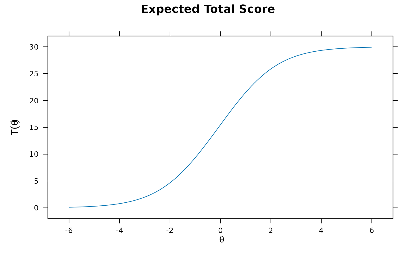plot(lltm, type = 'trace')

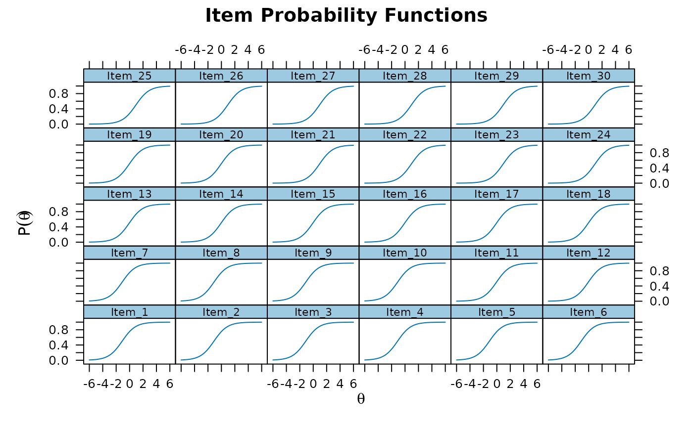itemplot(lltm, item=1)

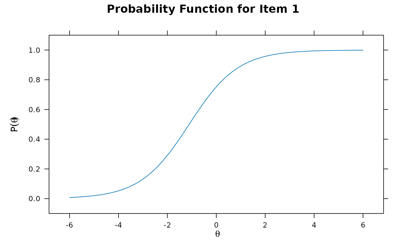itemfit(lltm)
#>       item   S_X2 df.S_X2 RMSEA.S_X2 p.S_X2
#> 1   Item_1 37.503      20      0.030  0.010
#> 2   Item_2 17.256      20      0.000  0.636
#> 3   Item_3 20.460      20      0.005  0.430
#> 4   Item_4 18.881      20      0.000  0.530
#> 5   Item_5 17.973      20      0.000  0.589
#> 6   Item_6 17.917      20      0.000  0.593
#> 7   Item_7 26.019      20      0.017  0.165
#> 8   Item_8 18.207      20      0.000  0.574
#> 9   Item_9 23.967      20      0.014  0.244
#> 10 Item_10 27.235      20      0.019  0.129
#> 11 Item_11 30.173      21      0.021  0.089
#> 12 Item_12 22.983      21      0.010  0.345
#> 13 Item_13 21.678      21      0.006  0.418
#> 14 Item_14 21.145      21      0.003  0.450
#> 15 Item_15 22.156      21      0.007  0.391
#> 16 Item_16 24.992      21      0.014  0.248
#> 17 Item_17 22.657      21      0.009  0.363
#> 18 Item_18 24.573      21      0.013  0.266
#> 19 Item_19 18.289      21      0.000  0.631
#> 20 Item_20 19.318      21      0.000  0.565
#> 21 Item_21 16.685      20      0.000  0.673
#> 22 Item_22 40.102      20      0.032  0.005
#> 23 Item_23 20.903      20      0.007  0.403
#> 24 Item_24 17.779      20      0.000  0.602
#> 25 Item_25 22.374      20      0.011  0.321
#> 26 Item_26 15.641      20      0.000  0.739
#> 27 Item_27 31.030      20      0.023  0.055
#> 28 Item_28 20.826      20      0.006  0.407
#> 29 Item_29 21.525      20      0.009  0.367
#> 30 Item_30 17.028      20      0.000  0.651
head(fscores(lltm))  #EAP estimates
#>              F1
#> [1,]  0.5464076
#> [2,]  0.4070378
#> [3,]  1.1433896
#> [4,] -1.6766429
#> [5,] -0.5496531
#> [6,] -0.1367036
fscores(lltm, method='EAPsum', full.scores=FALSE)
#>       df     X2  p.X2 SEM.alpha rxx.alpha rxx_F1
#> stats 28 23.142 0.726     2.392     0.844   0.84
#> 
#>    Sum.Scores     F1 SE_F1 observed expected std.res
#> 0           0 -2.638 0.552        0    0.962   0.981
#> 1           1 -2.354 0.515        2    3.223   0.681
#> 2           2 -2.104 0.485        6    6.686   0.265
#> 3           3 -1.880 0.461       10   11.099   0.330
#> 4           4 -1.677 0.442       12   16.180   1.039
#> 5           5 -1.489 0.426       27   21.661   1.147
#> 6           6 -1.313 0.412       31   27.306   0.707
#> 7           7 -1.148 0.402       29   32.904   0.681
#> 8           8 -0.990 0.393       45   38.271   1.088
#> 9           9 -0.839 0.386       46   43.246   0.419
#> 10         10 -0.692 0.380       44   47.691   0.534
#> 11         11 -0.550 0.375       57   51.486   0.768
#> 12         12 -0.410 0.372       55   54.536   0.063
#> 13         13 -0.273 0.370       48   56.766   1.164
#> 14         14 -0.137 0.368       58   58.123   0.016
#> 15         15 -0.001 0.368       46   58.575   1.643
#> 16         16  0.134 0.368       76   58.114   2.346
#> 17         17  0.270 0.369       57   56.753   0.033
#> 18         18  0.407 0.372       64   54.526   1.283
#> 19         19  0.546 0.375       49   51.488   0.347
#> 20         20  0.689 0.380       42   47.715   0.827
#> 21         21  0.835 0.385       42   43.301   0.198
#> 22         22  0.986 0.392       35   38.361   0.543
#> 23         23  1.143 0.401       30   33.029   0.527
#> 24         24  1.309 0.412       23   27.461   0.851
#> 25         25  1.484 0.425       20   21.834   0.393
#> 26         26  1.671 0.441       17   16.354   0.160
#> 27         27  1.875 0.461       13   11.256   0.520
#> 28         28  2.098 0.485        9    6.806   0.841
#> 29         29  2.348 0.515        6    3.295   1.490
#> 30         30  2.632 0.552        1    0.989   0.011
M2(lltm) # goodness of fit
#>             M2  df         p       RMSEA RMSEA_5   RMSEA_95      SRMSR
#> stats 474.3017 461 0.3242562 0.005374281       0 0.01222807 0.03141155
#>             TLI       CFI
#> stats 0.9987575 0.9986832
head(personfit(lltm))
#>      outfit   z.outfit     infit    z.infit        Zh
#> 1 0.9423934 -0.2421292 0.9198961 -0.4979024 0.4535529
#> 2 0.7498397 -1.5115718 0.8121325 -1.3393979 1.3472796
#> 3 0.9352178 -0.1230665 0.9381862 -0.2530007 0.2827676
#> 4 0.8654958 -0.1912980 0.7846585 -0.7460247 0.6570882
#> 5 0.7955355 -1.0902802 0.7561789 -1.6953154 1.4198055
#> 6 0.9599715 -0.2127795 0.9662941 -0.1961141 0.2470539
residuals(lltm)
#> LD matrix (lower triangle) and standardized residual correlations (upper triangle)
#> 
#> Upper triangle summary:
#>    Min. 1st Qu.  Median    Mean 3rd Qu.    Max. 
#>  -0.096  -0.042   0.014  -0.001   0.040   0.101 
#> 
#>         Item_1 Item_2 Item_3 Item_4 Item_5 Item_6 Item_7 Item_8 Item_9 Item_10
#> Item_1         -0.062 -0.075 -0.067 -0.052 -0.065 -0.056  0.055 -0.067  -0.065
#> Item_2   3.870         0.060 -0.049  0.024  0.018 -0.031 -0.018  0.017  -0.096
#> Item_3   5.658  3.555         0.025 -0.042  0.045 -0.033  0.023 -0.038  -0.079
#> Item_4   4.476  2.448  0.608        -0.044  0.033 -0.029 -0.031 -0.033  -0.061
#> Item_5   2.713  0.590  1.777  1.893         0.028 -0.029 -0.031  0.032   0.033
#> Item_6   4.200  0.309  2.045  1.101  0.758         0.042  0.027  0.018   0.040
#> Item_7   3.123  0.982  1.081  0.815  0.836  1.772        -0.039 -0.062  -0.037
#> Item_8   3.052  0.311  0.541  0.976  0.946  0.738  1.498         0.036  -0.041
#> Item_9   4.468  0.289  1.420  1.094  1.029  0.312  3.862  1.272         -0.052
#> Item_10  4.249  9.296  6.252  3.692  1.104  1.615  1.345  1.642  2.712        
#> Item_11  4.876  1.847  2.194  1.702  0.442  0.587  1.767  1.289  4.033   2.480
#> Item_12  2.511  0.708  0.222  1.124  0.219  8.541  0.516  0.343  0.961   2.162
#> Item_13  4.050  3.112  3.806  2.398  2.976  1.435  1.666  3.977  1.645   5.981
#> Item_14  2.873  0.347  0.300  3.435  0.203  0.259  7.592  0.196  0.286   1.922
#> Item_15  3.847  1.192  0.641  1.040  0.800  6.463  1.052  0.939  2.418   2.558
#> Item_16  4.525  0.762  1.585  1.366  4.307  0.496  0.696  0.541  0.516   2.459
#> Item_17  2.984  2.135  0.518  1.252  0.518  0.635  0.803  1.216  0.960   1.279
#> Item_18  3.408  0.222  0.112  0.611  0.768  2.580  1.194  0.189  1.337   2.636
#> Item_19  3.179  0.313  1.133  0.832  0.437  1.226  1.166  0.235  0.202   1.083
#> Item_20  6.900  1.506  3.056  2.474  1.557  3.595  1.865  1.903  1.774   4.484
#> Item_21  2.742  2.518  1.055  2.071  2.432  3.678  1.775  5.766  0.861   1.207
#> Item_22  3.467  1.804  0.510  1.569  2.332  0.618  7.319  0.981  2.212   5.397
#> Item_23  3.373  1.359  1.978  3.283  2.139  1.594  1.906  2.109  3.899   2.137
#> Item_24  4.731  0.186  0.150  1.907  0.150  0.214  0.737  2.373  6.674   2.045
#> Item_25  6.139  0.559  0.509  1.345  3.342  0.481  3.185  0.337  7.858   1.950
#> Item_26  2.771  1.794  0.208  3.581  0.317  1.184  0.404  0.837  3.259   2.408
#> Item_27  4.333  0.308  0.205  2.331  1.212  2.720  0.370  0.316  0.358   5.764
#> Item_28  6.039  2.035  1.252  1.939  1.726  3.961  1.360  1.634  1.386   3.003
#> Item_29  5.316  2.826  1.939  2.425  2.275  2.921  5.501  2.921  1.979   3.606
#> Item_30  3.375  0.900  0.135  1.740  0.690  1.932  0.294  0.280  2.730   1.112
#>         Item_11 Item_12 Item_13 Item_14 Item_15 Item_16 Item_17 Item_18 Item_19
#> Item_1   -0.070   0.050  -0.064  -0.054   0.062  -0.067  -0.055  -0.058  -0.056
#> Item_2   -0.043  -0.027   0.056  -0.019   0.035   0.028  -0.046  -0.015   0.018
#> Item_3    0.047  -0.015   0.062   0.017   0.025  -0.040  -0.023  -0.011   0.034
#> Item_4   -0.041   0.034   0.049  -0.059   0.032   0.037   0.035   0.025  -0.029
#> Item_5    0.021   0.015  -0.055   0.014   0.028   0.066  -0.023   0.028   0.021
#> Item_6   -0.024  -0.092   0.038   0.016   0.080   0.022   0.025   0.051   0.035
#> Item_7   -0.042   0.023  -0.041  -0.087   0.032  -0.026   0.028   0.035  -0.034
#> Item_8   -0.036   0.019   0.063   0.014  -0.031  -0.023  -0.035   0.014   0.015
#> Item_9   -0.064  -0.031  -0.041   0.017   0.049  -0.023  -0.031  -0.037  -0.014
#> Item_10  -0.050  -0.046  -0.077  -0.044  -0.051  -0.050   0.036  -0.051   0.033
#> Item_11          -0.030   0.047  -0.028  -0.034  -0.027   0.058   0.022   0.064
#> Item_12   0.892           0.035  -0.067   0.032  -0.034  -0.024   0.035   0.033
#> Item_13   2.184   1.234           0.043  -0.048   0.053   0.047   0.038   0.038
#> Item_14   0.784   4.427   1.824          -0.039  -0.037  -0.026  -0.028   0.012
#> Item_15   1.132   1.053   2.345   1.520           0.040   0.041  -0.031   0.040
#> Item_16   0.705   1.170   2.827   1.396   1.609           0.062   0.027   0.061
#> Item_17   3.335   0.591   2.196   0.668   1.650   3.855          -0.023   0.066
#> Item_18   0.467   1.212   1.435   0.766   0.985   0.738   0.519           0.033
#> Item_19   4.052   1.122   1.426   0.147   1.629   3.734   4.381   1.057        
#> Item_20   2.255   2.427   2.748   1.803   2.372   2.475   2.708   1.588   1.723
#> Item_21   1.540   1.018   2.913   0.656   1.312   1.222   0.828   0.549   0.733
#> Item_22   1.350   0.542   1.427   0.654   2.315   1.156   1.309   0.883   1.267
#> Item_23   2.059   1.856   2.571   1.705   4.760   2.680   1.756   3.496   2.176
#> Item_24   1.361   0.592   1.328   0.485   1.936   0.768   0.611   0.961   0.209
#> Item_25   3.449   0.340   5.951   0.402   1.597   1.055   1.150   2.770   2.938
#> Item_26   2.256   0.388   1.396   0.485   0.867   0.583   0.880   0.552   4.140
#> Item_27   0.621   0.604   3.430   0.267   1.505   3.404   0.944   0.329   3.045
#> Item_28   2.632   2.713   2.895   2.013   4.311   2.877  10.273   1.449   8.610
#> Item_29   3.353   2.994   3.653   2.056   3.662   2.491   3.100   3.346   2.210
#> Item_30   0.774   0.395   1.833   0.181   0.770   0.406   0.740   1.852   1.422
#>         Item_20 Item_21 Item_22 Item_23 Item_24 Item_25 Item_26 Item_27 Item_28
#> Item_1   -0.083  -0.052  -0.059   0.058  -0.069  -0.078  -0.053   0.066  -0.078
#> Item_2    0.039   0.050  -0.042   0.037   0.014  -0.024  -0.042   0.018  -0.045
#> Item_3    0.055  -0.032  -0.023   0.044   0.012   0.023   0.014  -0.014   0.035
#> Item_4    0.050  -0.046  -0.040  -0.057  -0.044  -0.037   0.060  -0.048  -0.044
#> Item_5    0.039  -0.049   0.048  -0.046   0.012  -0.058   0.018   0.035  -0.042
#> Item_6    0.060   0.061  -0.025  -0.040   0.015  -0.022   0.034   0.052   0.063
#> Item_7   -0.043   0.042  -0.086  -0.044  -0.027  -0.056  -0.020   0.019  -0.037
#> Item_8   -0.044  -0.076   0.031  -0.046   0.049  -0.018  -0.029   0.018  -0.040
#> Item_9    0.042   0.029  -0.047  -0.062   0.082  -0.089   0.057   0.019   0.037
#> Item_10  -0.067   0.035  -0.073   0.046  -0.045  -0.044  -0.049   0.076  -0.055
#> Item_11   0.047  -0.039   0.037  -0.045   0.037  -0.059   0.047   0.025  -0.051
#> Item_12  -0.049  -0.032   0.023  -0.043   0.024  -0.018  -0.020   0.025  -0.052
#> Item_13   0.052  -0.054  -0.038  -0.051   0.036  -0.077  -0.037   0.059  -0.054
#> Item_14  -0.042  -0.026   0.026   0.041  -0.022   0.020  -0.022   0.016  -0.045
#> Item_15   0.049  -0.036   0.048   0.069   0.044   0.040  -0.029   0.039   0.066
#> Item_16   0.050  -0.035   0.034   0.052   0.028  -0.032  -0.024   0.058   0.054
#> Item_17   0.052  -0.029   0.036   0.042   0.025  -0.034   0.030   0.031   0.101
#> Item_18  -0.040   0.023   0.030   0.059  -0.031  -0.053   0.023  -0.018  -0.038
#> Item_19   0.042   0.027   0.036   0.047   0.014  -0.054   0.064   0.055   0.093
#> Item_20           0.045  -0.079  -0.049  -0.073  -0.065   0.051  -0.042   0.057
#> Item_21   2.039           0.028   0.047  -0.070   0.030   0.044   0.084   0.070
#> Item_22   6.206   0.797           0.040  -0.028   0.040  -0.025   0.034  -0.055
#> Item_23   2.437   2.227   1.617          -0.043   0.037  -0.037   0.052  -0.073
#> Item_24   5.304   4.968   0.772   1.884          -0.027   0.041  -0.047   0.040
#> Item_25   4.277   0.921   1.617   1.403   0.744          -0.024   0.022   0.044
#> Item_26   2.599   1.947   0.641   1.335   1.706   0.568           0.048   0.071
#> Item_27   1.795   7.038   1.135   2.680   2.181   0.470   2.259          -0.039
#> Item_28   3.279   4.858   3.035   5.388   1.573   1.936   5.014   1.490        
#> Item_29   4.659   2.858   4.648   3.883   3.412   3.970   3.412   4.785   2.840
#> Item_30   1.608   1.100   1.657   2.451   0.681   1.088   0.814   2.928   1.287
#>         Item_29 Item_30
#> Item_1    0.073   0.058
#> Item_2    0.053   0.030
#> Item_3    0.044  -0.012
#> Item_4   -0.049   0.042
#> Item_5    0.048   0.026
#> Item_6    0.054   0.044
#> Item_7   -0.074  -0.017
#> Item_8    0.054   0.017
#> Item_9   -0.044   0.052
#> Item_10   0.060   0.033
#> Item_11  -0.058  -0.028
#> Item_12  -0.055   0.020
#> Item_13   0.060   0.043
#> Item_14  -0.045  -0.013
#> Item_15   0.061   0.028
#> Item_16  -0.050  -0.020
#> Item_17   0.056  -0.027
#> Item_18  -0.058   0.043
#> Item_19  -0.047   0.038
#> Item_20  -0.068  -0.040
#> Item_21  -0.053  -0.033
#> Item_22  -0.068   0.041
#> Item_23   0.062   0.050
#> Item_24   0.058  -0.026
#> Item_25  -0.063  -0.033
#> Item_26   0.058   0.029
#> Item_27   0.069   0.054
#> Item_28  -0.053  -0.036
#> Item_29           0.083
#> Item_30   6.832        

# intercept across items also possible by removing ~ 0 portion, just interpreted differently
lltm.int <- mirt(dat, itemtype = 'Rasch',
   item.formula = ~ difficulty, itemdesign=itemdesign)
#> 
anova(lltm, lltm.int) # same
#>               AIC   SABIC       HQ     BIC    logLik X2 df   p
#> lltm     35429.67 35436.6 35437.13 35449.3 -17710.84          
#> lltm.int 35429.67 35436.6 35437.13 35449.3 -17710.84  0  0 NaN
coef(lltm.int, simplify=TRUE)
#> $items
#>         (Intercept) difficultyhard difficultymedium a1 d g u
#> Item_1        0.988           0.00            0.000  1 0 0 1
#> Item_2        0.988           0.00            0.000  1 0 0 1
#> Item_3        0.988           0.00            0.000  1 0 0 1
#> Item_4        0.988           0.00            0.000  1 0 0 1
#> Item_5        0.988           0.00            0.000  1 0 0 1
#> Item_6        0.988           0.00            0.000  1 0 0 1
#> Item_7        0.988           0.00            0.000  1 0 0 1
#> Item_8        0.988           0.00            0.000  1 0 0 1
#> Item_9        0.988           0.00            0.000  1 0 0 1
#> Item_10       0.988           0.00            0.000  1 0 0 1
#> Item_11       0.988           0.00           -1.004  1 0 0 1
#> Item_12       0.988           0.00           -1.004  1 0 0 1
#> Item_13       0.988           0.00           -1.004  1 0 0 1
#> Item_14       0.988           0.00           -1.004  1 0 0 1
#> Item_15       0.988           0.00           -1.004  1 0 0 1
#> Item_16       0.988           0.00           -1.004  1 0 0 1
#> Item_17       0.988           0.00           -1.004  1 0 0 1
#> Item_18       0.988           0.00           -1.004  1 0 0 1
#> Item_19       0.988           0.00           -1.004  1 0 0 1
#> Item_20       0.988           0.00           -1.004  1 0 0 1
#> Item_21       0.988          -1.95            0.000  1 0 0 1
#> Item_22       0.988          -1.95            0.000  1 0 0 1
#> Item_23       0.988          -1.95            0.000  1 0 0 1
#> Item_24       0.988          -1.95            0.000  1 0 0 1
#> Item_25       0.988          -1.95            0.000  1 0 0 1
#> Item_26       0.988          -1.95            0.000  1 0 0 1
#> Item_27       0.988          -1.95            0.000  1 0 0 1
#> Item_28       0.988          -1.95            0.000  1 0 0 1
#> Item_29       0.988          -1.95            0.000  1 0 0 1
#> Item_30       0.988          -1.95            0.000  1 0 0 1
#> 
#> $means
#> F1 
#>  0 
#> 
#> $cov
#>       F1
#> F1 0.948
#> 

# using unconditional modeling for first four items
itemdesign.sub <- itemdesign[5:nrow(itemdesign), , drop=FALSE]
itemdesign.sub    # note that rownames are required in this case
#>         difficulty
#> Item_5        easy
#> Item_6        easy
#> Item_7        easy
#> Item_8        easy
#> Item_9        easy
#> Item_10       easy
#> Item_11     medium
#> Item_12     medium
#> Item_13     medium
#> Item_14     medium
#> Item_15     medium
#> Item_16     medium
#> Item_17     medium
#> Item_18     medium
#> Item_19     medium
#> Item_20     medium
#> Item_21       hard
#> Item_22       hard
#> Item_23       hard
#> Item_24       hard
#> Item_25       hard
#> Item_26       hard
#> Item_27       hard
#> Item_28       hard
#> Item_29       hard
#> Item_30       hard
lltm.4 <- mirt(dat, itemtype = 'Rasch',
   item.formula = ~ 0 + difficulty, itemdesign=itemdesign.sub)
#> 
coef(lltm.4, simplify=TRUE) # first four items are the standard Rasch
#> $items
#>         difficultyeasy difficultyhard difficultymedium a1     d g u
#> Item_1           0.000          0.000            0.000  1 0.866 0 1
#> Item_2           0.000          0.000            0.000  1 0.969 0 1
#> Item_3           0.000          0.000            0.000  1 1.002 0 1
#> Item_4           0.000          0.000            0.000  1 1.053 0 1
#> Item_5           0.999          0.000            0.000  1 0.000 0 1
#> Item_6           0.999          0.000            0.000  1 0.000 0 1
#> Item_7           0.999          0.000            0.000  1 0.000 0 1
#> Item_8           0.999          0.000            0.000  1 0.000 0 1
#> Item_9           0.999          0.000            0.000  1 0.000 0 1
#> Item_10          0.999          0.000            0.000  1 0.000 0 1
#> Item_11          0.000          0.000           -0.016  1 0.000 0 1
#> Item_12          0.000          0.000           -0.016  1 0.000 0 1
#> Item_13          0.000          0.000           -0.016  1 0.000 0 1
#> Item_14          0.000          0.000           -0.016  1 0.000 0 1
#> Item_15          0.000          0.000           -0.016  1 0.000 0 1
#> Item_16          0.000          0.000           -0.016  1 0.000 0 1
#> Item_17          0.000          0.000           -0.016  1 0.000 0 1
#> Item_18          0.000          0.000           -0.016  1 0.000 0 1
#> Item_19          0.000          0.000           -0.016  1 0.000 0 1
#> Item_20          0.000          0.000           -0.016  1 0.000 0 1
#> Item_21          0.000         -0.961            0.000  1 0.000 0 1
#> Item_22          0.000         -0.961            0.000  1 0.000 0 1
#> Item_23          0.000         -0.961            0.000  1 0.000 0 1
#> Item_24          0.000         -0.961            0.000  1 0.000 0 1
#> Item_25          0.000         -0.961            0.000  1 0.000 0 1
#> Item_26          0.000         -0.961            0.000  1 0.000 0 1
#> Item_27          0.000         -0.961            0.000  1 0.000 0 1
#> Item_28          0.000         -0.961            0.000  1 0.000 0 1
#> Item_29          0.000         -0.961            0.000  1 0.000 0 1
#> Item_30          0.000         -0.961            0.000  1 0.000 0 1
#> 
#> $means
#> F1 
#>  0 
#> 
#> $cov
#>       F1
#> F1 0.948
#> 
anova(lltm, lltm.4) # similar fit, hence more constrained model preferred
#>             AIC    SABIC       HQ      BIC    logLik    X2 df     p
#> lltm   35429.67 35436.60 35437.13 35449.30 -17710.84               
#> lltm.4 35433.92 35447.78 35448.84 35473.18 -17708.96 3.751  4 0.441

# LLTM with mixedmirt() (more flexible in general, but slower)
LLTM <- mixedmirt(dat, model=1, fixed = ~ 0 + difficulty,
                  itemdesign=itemdesign, SE=FALSE)
#> , Max-Change = 0.1846, Max-Change = 0.1471, Max-Change = 0.1240, Max-Change = 0.0962, Max-Change = 0.0800, Max-Change = 0.0656, Max-Change = 0.0550, Max-Change = 0.0444, Max-Change = 0.0355, Max-Change = 0.0306, Max-Change = 0.0259, Max-Change = 0.0211, Max-Change = 0.0184, Max-Change = 0.0138, Max-Change = 0.0147, Max-Change = 0.0124, Max-Change = 0.0104, Max-Change = 0.0084, Max-Change = 0.0135, Max-Change = 0.0106, Max-Change = 0.0081, Max-Change = 0.0076, Max-Change = 0.0047, Max-Change = 0.0074, Max-Change = 0.0059, Max-Change = 0.0035, Max-Change = 0.0064, Max-Change = 0.0011, Max-Change = 0.0072, Max-Change = 0.0032, Max-Change = 0.0031, Max-Change = 0.0092, Max-Change = 0.0060, Max-Change = 0.0004, Max-Change = 0.0041, Max-Change = 0.0011, Max-Change = 0.0035, Max-Change = 0.0032, Max-Change = 0.0037, Max-Change = 0.0048, Max-Change = 0.0029, Max-Change = 0.0025, Max-Change = 0.0044, Max-Change = 0.0036, Max-Change = 0.0040, Max-Change = 0.0030, Max-Change = 0.0018, Max-Change = 0.0090, Max-Change = 0.0025, Max-Change = 0.0031, Max-Change = 0.0120, Max-Change = 0.0045, Max-Change = 0.0044, Max-Change = 0.0034, Max-Change = 0.0012, Max-Change = 0.0025, Max-Change = 0.0015, Max-Change = 0.0036, Max-Change = 0.0067, Max-Change = 0.0041, Max-Change = 0.0061, Max-Change = 0.0060, Max-Change = 0.0017, Max-Change = 0.0028, Max-Change = 0.0030, Max-Change = 0.0026, Max-Change = 0.0075, Max-Change = 0.0093, Max-Change = 0.0045, Max-Change = 0.0064, Max-Change = 0.0084, Max-Change = 0.0040, Max-Change = 0.0007, Max-Change = 0.0076, Max-Change = 0.0052, Max-Change = 0.0052, Max-Change = 0.0005, Max-Change = 0.0035, Max-Change = 0.0051, Max-Change = 0.0016, Max-Change = 0.0040, Max-Change = 0.0056, Max-Change = 0.0029, Max-Change = 0.0053, Max-Change = 0.0020, Max-Change = 0.0093, Max-Change = 0.0059, Max-Change = 0.0050, Max-Change = 0.0048, Max-Change = 0.0055, Max-Change = 0.0028, Max-Change = 0.0092, Max-Change = 0.0063, Max-Change = 0.0052, Max-Change = 0.0044, Max-Change = 0.0186, Max-Change = 0.0019, Max-Change = 0.0042, Max-Change = 0.0142, Max-Change = 0.0091, Max-Change = 0.0038, Max-Change = 0.0040, Max-Change = 0.0033, Max-Change = 0.0043, Max-Change = 0.0014, Max-Change = 0.0040, Max-Change = 0.0044, Max-Change = 0.0055, Max-Change = 0.0061, Max-Change = 0.0038, Max-Change = 0.0079, Max-Change = 0.0027, Max-Change = 0.0037, Max-Change = 0.0072, Max-Change = 0.0077, Max-Change = 0.0045, Max-Change = 0.0034, Max-Change = 0.0049, Max-Change = 0.0047, Max-Change = 0.0034, Max-Change = 0.0045, Max-Change = 0.0022, Max-Change = 0.0037, Max-Change = 0.0079, Max-Change = 0.0045, Max-Change = 0.0093, Max-Change = 0.0015, Max-Change = 0.0032, Max-Change = 0.0078, Max-Change = 0.0040, Max-Change = 0.0080, Max-Change = 0.0055, Max-Change = 0.0086, Max-Change = 0.0056, Max-Change = 0.0006, Max-Change = 0.0067, Max-Change = 0.0052, Max-Change = 0.0012, Max-Change = 0.0126, Max-Change = 0.0080, Max-Change = 0.0017, Max-Change = 0.0033, Max-Change = 0.0053, Max-Change = 0.0027, Max-Change = 0.0106, Max-Change = 0.0011, Max-Change = 0.0098, Max-Change = 0.0035, Max-Change = 0.0053, Max-Change = 0.0067, Max-Change = 0.0025, Max-Change = 0.0089, Max-Change = 0.0103, Max-Change = 0.0017, Max-Change = 0.0032, Max-Change = 0.0083, Max-Change = 0.0035, Max-Change = 0.0016, Max-Change = 0.0038, Max-Change = 0.0107, Max-Change = 0.0016, Max-Change = 0.0128, Max-Change = 0.0056, Max-Change = 0.0042, Max-Change = 0.0044, Max-Change = 0.0030, Max-Change = 0.0030, Max-Change = 0.0054, Max-Change = 0.0053, Max-Change = 0.0018, Max-Change = 0.0014, Max-Change = 0.0015, Max-Change = 0.0020, Max-Change = 0.0042, Max-Change = 0.0050, Max-Change = 0.0039, Max-Change = 0.0061, Max-Change = 0.0021, Max-Change = 0.0109, Max-Change = 0.0018, Max-Change = 0.0022, Max-Change = 0.0042, Max-Change = 0.0045, Max-Change = 0.0012, Max-Change = 0.0009, Max-Change = 0.0019, Max-Change = 0.0003, Max-Change = 0.0059, Max-Change = 0.0062, Max-Change = 0.0028, Max-Change = 0.0047, Max-Change = 0.0031, Max-Change = 0.0015, Max-Change = 0.0040, Max-Change = 0.0020, Max-Change = 0.0045, Max-Change = 0.0034, Max-Change = 0.0002, Max-Change = 0.0017, Max-Change = 0.0060, Max-Change = 0.0052, Max-Change = 0.0021, Max-Change = 0.0013, Max-Change = 0.0031, Max-Change = 0.0102, Max-Change = 0.0078, Max-Change = 0.0047, Max-Change = 0.0037, Max-Change = 0.0060, Max-Change = 0.0070, Max-Change = 0.0031, Max-Change = 0.0040, Max-Change = 0.0053, Max-Change = 0.0043, Max-Change = 0.0032, Max-Change = 0.0038, Max-Change = 0.0083, Max-Change = 0.0017, Max-Change = 0.0024, Max-Change = 0.0053, Max-Change = 0.0053, Max-Change = 0.0054, Max-Change = 0.0021, Max-Change = 0.0029, Max-Change = 0.0057, Max-Change = 0.0091, Max-Change = 0.0050, Max-Change = 0.0054, Max-Change = 0.0034, Max-Change = 0.0089, Max-Change = 0.0033, Max-Change = 0.0098, Max-Change = 0.0013, Max-Change = 0.0082, Max-Change = 0.0029, Max-Change = 0.0027, Max-Change = 0.0022, Max-Change = 0.0051, Max-Change = 0.0038, Max-Change = 0.0034, Max-Change = 0.0027, Max-Change = 0.0021, Max-Change = 0.0048, Max-Change = 0.0022, Max-Change = 0.0033, Max-Change = 0.0044, Max-Change = 0.0086, Max-Change = 0.0032, Max-Change = 0.0058, Max-Change = 0.0070, gam = 0.0000, Max-Change = 0.0000, gam = 0.1778, Max-Change = 0.0022, gam = 0.1057, Max-Change = 0.0046, gam = 0.0780, Max-Change = 0.0032, gam = 0.0629, Max-Change = 0.0023, gam = 0.0532, Max-Change = 0.0013, gam = 0.0464, Max-Change = 0.0006, gam = 0.0413, Max-Change = 0.0005, gam = 0.0374, Max-Change = 0.0013, gam = 0.0342, Max-Change = 0.0022, gam = 0.0316, Max-Change = 0.0010, gam = 0.0294, Max-Change = 0.0006, gam = 0.0276, Max-Change = 0.0001

#> 
#> Calculating log-likelihood...
summary(LLTM)
#> 
#> Call:
#> mixedmirt(data = dat, model = 1, fixed = ~0 + difficulty, itemdesign = itemdesign, 
#>     SE = FALSE)
#> 
#> --------------
#> FIXED EFFECTS:
#>                  Estimate Std.Error z.value
#> difficultyeasy      0.993        NA      NA
#> difficultyhard     -0.956        NA      NA
#> difficultymedium   -0.012        NA      NA
#> 
#> --------------
#> RANDOM EFFECT COVARIANCE(S):
#> Correlations on upper diagonal
#> 
#> $Theta
#>       F1
#> F1 0.945
#> 
coef(LLTM)
#> $Item_1
#>     difficultyeasy difficultyhard difficultymedium a1 d g u
#> par          0.993         -0.956           -0.012  1 0 0 1
#> 
#> $Item_2
#>     difficultyeasy difficultyhard difficultymedium a1 d g u
#> par          0.993         -0.956           -0.012  1 0 0 1
#> 
#> $Item_3
#>     difficultyeasy difficultyhard difficultymedium a1 d g u
#> par          0.993         -0.956           -0.012  1 0 0 1
#> 
#> $Item_4
#>     difficultyeasy difficultyhard difficultymedium a1 d g u
#> par          0.993         -0.956           -0.012  1 0 0 1
#> 
#> $Item_5
#>     difficultyeasy difficultyhard difficultymedium a1 d g u
#> par          0.993         -0.956           -0.012  1 0 0 1
#> 
#> $Item_6
#>     difficultyeasy difficultyhard difficultymedium a1 d g u
#> par          0.993         -0.956           -0.012  1 0 0 1
#> 
#> $Item_7
#>     difficultyeasy difficultyhard difficultymedium a1 d g u
#> par          0.993         -0.956           -0.012  1 0 0 1
#> 
#> $Item_8
#>     difficultyeasy difficultyhard difficultymedium a1 d g u
#> par          0.993         -0.956           -0.012  1 0 0 1
#> 
#> $Item_9
#>     difficultyeasy difficultyhard difficultymedium a1 d g u
#> par          0.993         -0.956           -0.012  1 0 0 1
#> 
#> $Item_10
#>     difficultyeasy difficultyhard difficultymedium a1 d g u
#> par          0.993         -0.956           -0.012  1 0 0 1
#> 
#> $Item_11
#>     difficultyeasy difficultyhard difficultymedium a1 d g u
#> par          0.993         -0.956           -0.012  1 0 0 1
#> 
#> $Item_12
#>     difficultyeasy difficultyhard difficultymedium a1 d g u
#> par          0.993         -0.956           -0.012  1 0 0 1
#> 
#> $Item_13
#>     difficultyeasy difficultyhard difficultymedium a1 d g u
#> par          0.993         -0.956           -0.012  1 0 0 1
#> 
#> $Item_14
#>     difficultyeasy difficultyhard difficultymedium a1 d g u
#> par          0.993         -0.956           -0.012  1 0 0 1
#> 
#> $Item_15
#>     difficultyeasy difficultyhard difficultymedium a1 d g u
#> par          0.993         -0.956           -0.012  1 0 0 1
#> 
#> $Item_16
#>     difficultyeasy difficultyhard difficultymedium a1 d g u
#> par          0.993         -0.956           -0.012  1 0 0 1
#> 
#> $Item_17
#>     difficultyeasy difficultyhard difficultymedium a1 d g u
#> par          0.993         -0.956           -0.012  1 0 0 1
#> 
#> $Item_18
#>     difficultyeasy difficultyhard difficultymedium a1 d g u
#> par          0.993         -0.956           -0.012  1 0 0 1
#> 
#> $Item_19
#>     difficultyeasy difficultyhard difficultymedium a1 d g u
#> par          0.993         -0.956           -0.012  1 0 0 1
#> 
#> $Item_20
#>     difficultyeasy difficultyhard difficultymedium a1 d g u
#> par          0.993         -0.956           -0.012  1 0 0 1
#> 
#> $Item_21
#>     difficultyeasy difficultyhard difficultymedium a1 d g u
#> par          0.993         -0.956           -0.012  1 0 0 1
#> 
#> $Item_22
#>     difficultyeasy difficultyhard difficultymedium a1 d g u
#> par          0.993         -0.956           -0.012  1 0 0 1
#> 
#> $Item_23
#>     difficultyeasy difficultyhard difficultymedium a1 d g u
#> par          0.993         -0.956           -0.012  1 0 0 1
#> 
#> $Item_24
#>     difficultyeasy difficultyhard difficultymedium a1 d g u
#> par          0.993         -0.956           -0.012  1 0 0 1
#> 
#> $Item_25
#>     difficultyeasy difficultyhard difficultymedium a1 d g u
#> par          0.993         -0.956           -0.012  1 0 0 1
#> 
#> $Item_26
#>     difficultyeasy difficultyhard difficultymedium a1 d g u
#> par          0.993         -0.956           -0.012  1 0 0 1
#> 
#> $Item_27
#>     difficultyeasy difficultyhard difficultymedium a1 d g u
#> par          0.993         -0.956           -0.012  1 0 0 1
#> 
#> $Item_28
#>     difficultyeasy difficultyhard difficultymedium a1 d g u
#> par          0.993         -0.956           -0.012  1 0 0 1
#> 
#> $Item_29
#>     difficultyeasy difficultyhard difficultymedium a1 d g u
#> par          0.993         -0.956           -0.012  1 0 0 1
#> 
#> $Item_30
#>     difficultyeasy difficultyhard difficultymedium a1 d g u
#> par          0.993         -0.956           -0.012  1 0 0 1
#> 
#> $GroupPars
#>     MEAN_1 COV_11
#> par      0  0.945
#> 

# LLTM with random error estimate (not supported with mirt() )
LLTM.e <- mixedmirt(dat, model=1, fixed = ~ 0 + difficulty,
                  random = ~ 1|items, itemdesign=itemdesign, SE=FALSE)
#> , Max-Change = 0.1846, Max-Change = 0.1471, Max-Change = 0.1240, Max-Change = 0.0962, Max-Change = 0.0800, Max-Change = 0.0656, Max-Change = 0.0550, Max-Change = 0.0444, Max-Change = 0.0355, Max-Change = 0.0306, Max-Change = 0.0259, Max-Change = 0.0211, Max-Change = 0.0184, Max-Change = 0.0138, Max-Change = 0.0147, Max-Change = 0.0124, Max-Change = 0.0104, Max-Change = 0.0084, Max-Change = 0.0135, Max-Change = 0.0106, Max-Change = 0.0081, Max-Change = 0.0076, Max-Change = 0.0047, Max-Change = 0.0074, Max-Change = 0.0059, Max-Change = 0.0035, Max-Change = 0.0064, Max-Change = 0.0011, Max-Change = 0.0072, Max-Change = 0.0032, Max-Change = 0.0031, Max-Change = 0.0092, Max-Change = 0.0060, Max-Change = 0.0004, Max-Change = 0.0041, Max-Change = 0.0011, Max-Change = 0.0035, Max-Change = 0.0032, Max-Change = 0.0037, Max-Change = 0.0048, Max-Change = 0.0029, Max-Change = 0.0025, Max-Change = 0.0044, Max-Change = 0.0036, Max-Change = 0.0040, Max-Change = 0.0030, Max-Change = 0.0018, Max-Change = 0.0090, Max-Change = 0.0025, Max-Change = 0.0031, Max-Change = 0.0120, Max-Change = 0.0045, Max-Change = 0.0044, Max-Change = 0.0034, Max-Change = 0.0012, Max-Change = 0.0025, Max-Change = 0.0015, Max-Change = 0.0036, Max-Change = 0.0067, Max-Change = 0.0041, Max-Change = 0.0061, Max-Change = 0.0060, Max-Change = 0.0017, Max-Change = 0.0028, Max-Change = 0.0030, Max-Change = 0.0026, Max-Change = 0.0075, Max-Change = 0.0093, Max-Change = 0.0045, Max-Change = 0.0064, Max-Change = 0.0084, Max-Change = 0.0040, Max-Change = 0.0007, Max-Change = 0.0076, Max-Change = 0.0052, Max-Change = 0.0052, Max-Change = 0.0005, Max-Change = 0.0035, Max-Change = 0.0051, Max-Change = 0.0016, Max-Change = 0.0040, Max-Change = 0.0056, Max-Change = 0.0029, Max-Change = 0.0053, Max-Change = 0.0020, Max-Change = 0.0093, Max-Change = 0.0059, Max-Change = 0.0050, Max-Change = 0.0048, Max-Change = 0.0055, Max-Change = 0.0028, Max-Change = 0.0092, Max-Change = 0.0063, Max-Change = 0.0052, Max-Change = 0.0044, Max-Change = 0.0186, Max-Change = 0.0019, Max-Change = 0.0042, Max-Change = 0.0142, Max-Change = 0.0284, Max-Change = 0.2000, Max-Change = 0.1627, Max-Change = 0.1300, Max-Change = 0.1035, Max-Change = 0.0832, Max-Change = 0.0664, Max-Change = 0.0534, Max-Change = 0.0433, Max-Change = 0.0345, Max-Change = 0.0281, Max-Change = 0.0215, Max-Change = 0.0175, Max-Change = 0.0162, Max-Change = 0.0150, Max-Change = 0.0397, Max-Change = 0.0031, Max-Change = 0.0014, Max-Change = 0.0065, Max-Change = 0.0030, Max-Change = 0.0064, Max-Change = 0.0038, Max-Change = 0.0116, Max-Change = 0.0053, Max-Change = 0.0034, Max-Change = 0.0054, Max-Change = 0.0043, Max-Change = 0.0111, Max-Change = 0.0052, Max-Change = 0.0020, Max-Change = 0.0083, Max-Change = 0.0068, Max-Change = 0.0052, Max-Change = 0.0052, Max-Change = 0.0048, Max-Change = 0.0057, Max-Change = 0.0057, Max-Change = 0.0025, Max-Change = 0.0042, Max-Change = 0.0066, Max-Change = 0.0081, Max-Change = 0.0048, Max-Change = 0.0027, Max-Change = 0.0057, Max-Change = 0.0046, Max-Change = 0.0040, Max-Change = 0.0040, Max-Change = 0.0052, Max-Change = 0.0080, Max-Change = 0.0037, Max-Change = 0.0052, Max-Change = 0.0070, Max-Change = 0.0012, Max-Change = 0.0066, Max-Change = 0.0062, Max-Change = 0.0040, Max-Change = 0.0053, Max-Change = 0.0051, Max-Change = 0.0076, Max-Change = 0.0033, Max-Change = 0.0038, Max-Change = 0.0047, Max-Change = 0.0037, Max-Change = 0.0075, Max-Change = 0.0066, Max-Change = 0.0057, Max-Change = 0.0023, Max-Change = 0.0015, Max-Change = 0.0042, Max-Change = 0.0037, Max-Change = 0.0063, Max-Change = 0.0092, Max-Change = 0.0016, Max-Change = 0.0082, Max-Change = 0.0018, Max-Change = 0.0064, Max-Change = 0.0054, Max-Change = 0.0031, Max-Change = 0.0060, Max-Change = 0.0027, Max-Change = 0.0070, Max-Change = 0.0072, Max-Change = 0.0020, Max-Change = 0.0052, Max-Change = 0.0068, Max-Change = 0.0055, Max-Change = 0.0036, Max-Change = 0.0049, Max-Change = 0.0078, Max-Change = 0.0026, Max-Change = 0.0059, Max-Change = 0.0020, Max-Change = 0.0029, Max-Change = 0.0057, Max-Change = 0.0077, Max-Change = 0.0030, Max-Change = 0.0023, Max-Change = 0.0041, Max-Change = 0.0050, Max-Change = 0.0033, Max-Change = 0.0127, Max-Change = 0.0056, Max-Change = 0.0077, Max-Change = 0.0054, Max-Change = 0.0045, Max-Change = 0.0042, Max-Change = 0.0020, Max-Change = 0.0068, Max-Change = 0.0065, Max-Change = 0.0021, Max-Change = 0.0026, Max-Change = 0.0041, Max-Change = 0.0109, Max-Change = 0.0061, Max-Change = 0.0106, Max-Change = 0.0026, Max-Change = 0.0061, Max-Change = 0.0072, Max-Change = 0.0076, Max-Change = 0.0053, Max-Change = 0.0076, Max-Change = 0.0140, Max-Change = 0.0019, Max-Change = 0.0026, Max-Change = 0.0032, Max-Change = 0.0021, Max-Change = 0.0047, Max-Change = 0.0043, Max-Change = 0.0016, Max-Change = 0.0086, Max-Change = 0.0033, Max-Change = 0.0052, Max-Change = 0.0138, Max-Change = 0.0038, Max-Change = 0.0032, Max-Change = 0.0070, Max-Change = 0.0060, Max-Change = 0.0070, Max-Change = 0.0025, Max-Change = 0.0015, Max-Change = 0.0042, Max-Change = 0.0034, Max-Change = 0.0023, Max-Change = 0.0035, Max-Change = 0.0063, Max-Change = 0.0057, Max-Change = 0.0042, Max-Change = 0.0063, Max-Change = 0.0058, Max-Change = 0.0017, Max-Change = 0.0079, Max-Change = 0.0085, Max-Change = 0.0072, Max-Change = 0.0031, Max-Change = 0.0048, Max-Change = 0.0064, Max-Change = 0.0029, Max-Change = 0.0048, Max-Change = 0.0018, Max-Change = 0.0050, Max-Change = 0.0035, Max-Change = 0.0069, Max-Change = 0.0008, Max-Change = 0.0052, Max-Change = 0.0023, Max-Change = 0.0009, Max-Change = 0.0031, Max-Change = 0.0103, Max-Change = 0.0048, Max-Change = 0.0027, Max-Change = 0.0055, Max-Change = 0.0118, Max-Change = 0.0031, Max-Change = 0.0029, Max-Change = 0.0044, Max-Change = 0.0058, Max-Change = 0.0008, Max-Change = 0.0053, Max-Change = 0.0047, Max-Change = 0.0005, Max-Change = 0.0041, Max-Change = 0.0054, Max-Change = 0.0030, Max-Change = 0.0016, Max-Change = 0.0067, Max-Change = 0.0064, Max-Change = 0.0060, Max-Change = 0.0025, Max-Change = 0.0058, Max-Change = 0.0070, Max-Change = 0.0038, Max-Change = 0.0054, Max-Change = 0.0041, Max-Change = 0.0053, Max-Change = 0.0043, Max-Change = 0.0071, Max-Change = 0.0012, Max-Change = 0.0028, Max-Change = 0.0045, Max-Change = 0.0031, Max-Change = 0.0028, gam = 0.0000, Max-Change = 0.0000, gam = 0.1778, Max-Change = 0.0053, gam = 0.1057, Max-Change = 0.0015, gam = 0.0780, Max-Change = 0.0023, gam = 0.0629, Max-Change = 0.0020, gam = 0.0532, Max-Change = 0.0008, gam = 0.0464, Max-Change = 0.0001, gam = 0.0413, Max-Change = 0.0004

#> 
#> Calculating log-likelihood...
coef(LLTM.e)
#> $Item_1
#>     difficultyeasy difficultyhard difficultymedium a1 d g u
#> par          1.003         -0.964             0.01  1 0 0 1
#> 
#> $Item_2
#>     difficultyeasy difficultyhard difficultymedium a1 d g u
#> par          1.003         -0.964             0.01  1 0 0 1
#> 
#> $Item_3
#>     difficultyeasy difficultyhard difficultymedium a1 d g u
#> par          1.003         -0.964             0.01  1 0 0 1
#> 
#> $Item_4
#>     difficultyeasy difficultyhard difficultymedium a1 d g u
#> par          1.003         -0.964             0.01  1 0 0 1
#> 
#> $Item_5
#>     difficultyeasy difficultyhard difficultymedium a1 d g u
#> par          1.003         -0.964             0.01  1 0 0 1
#> 
#> $Item_6
#>     difficultyeasy difficultyhard difficultymedium a1 d g u
#> par          1.003         -0.964             0.01  1 0 0 1
#> 
#> $Item_7
#>     difficultyeasy difficultyhard difficultymedium a1 d g u
#> par          1.003         -0.964             0.01  1 0 0 1
#> 
#> $Item_8
#>     difficultyeasy difficultyhard difficultymedium a1 d g u
#> par          1.003         -0.964             0.01  1 0 0 1
#> 
#> $Item_9
#>     difficultyeasy difficultyhard difficultymedium a1 d g u
#> par          1.003         -0.964             0.01  1 0 0 1
#> 
#> $Item_10
#>     difficultyeasy difficultyhard difficultymedium a1 d g u
#> par          1.003         -0.964             0.01  1 0 0 1
#> 
#> $Item_11
#>     difficultyeasy difficultyhard difficultymedium a1 d g u
#> par          1.003         -0.964             0.01  1 0 0 1
#> 
#> $Item_12
#>     difficultyeasy difficultyhard difficultymedium a1 d g u
#> par          1.003         -0.964             0.01  1 0 0 1
#> 
#> $Item_13
#>     difficultyeasy difficultyhard difficultymedium a1 d g u
#> par          1.003         -0.964             0.01  1 0 0 1
#> 
#> $Item_14
#>     difficultyeasy difficultyhard difficultymedium a1 d g u
#> par          1.003         -0.964             0.01  1 0 0 1
#> 
#> $Item_15
#>     difficultyeasy difficultyhard difficultymedium a1 d g u
#> par          1.003         -0.964             0.01  1 0 0 1
#> 
#> $Item_16
#>     difficultyeasy difficultyhard difficultymedium a1 d g u
#> par          1.003         -0.964             0.01  1 0 0 1
#> 
#> $Item_17
#>     difficultyeasy difficultyhard difficultymedium a1 d g u
#> par          1.003         -0.964             0.01  1 0 0 1
#> 
#> $Item_18
#>     difficultyeasy difficultyhard difficultymedium a1 d g u
#> par          1.003         -0.964             0.01  1 0 0 1
#> 
#> $Item_19
#>     difficultyeasy difficultyhard difficultymedium a1 d g u
#> par          1.003         -0.964             0.01  1 0 0 1
#> 
#> $Item_20
#>     difficultyeasy difficultyhard difficultymedium a1 d g u
#> par          1.003         -0.964             0.01  1 0 0 1
#> 
#> $Item_21
#>     difficultyeasy difficultyhard difficultymedium a1 d g u
#> par          1.003         -0.964             0.01  1 0 0 1
#> 
#> $Item_22
#>     difficultyeasy difficultyhard difficultymedium a1 d g u
#> par          1.003         -0.964             0.01  1 0 0 1
#> 
#> $Item_23
#>     difficultyeasy difficultyhard difficultymedium a1 d g u
#> par          1.003         -0.964             0.01  1 0 0 1
#> 
#> $Item_24
#>     difficultyeasy difficultyhard difficultymedium a1 d g u
#> par          1.003         -0.964             0.01  1 0 0 1
#> 
#> $Item_25
#>     difficultyeasy difficultyhard difficultymedium a1 d g u
#> par          1.003         -0.964             0.01  1 0 0 1
#> 
#> $Item_26
#>     difficultyeasy difficultyhard difficultymedium a1 d g u
#> par          1.003         -0.964             0.01  1 0 0 1
#> 
#> $Item_27
#>     difficultyeasy difficultyhard difficultymedium a1 d g u
#> par          1.003         -0.964             0.01  1 0 0 1
#> 
#> $Item_28
#>     difficultyeasy difficultyhard difficultymedium a1 d g u
#> par          1.003         -0.964             0.01  1 0 0 1
#> 
#> $Item_29
#>     difficultyeasy difficultyhard difficultymedium a1 d g u
#> par          1.003         -0.964             0.01  1 0 0 1
#> 
#> $Item_30
#>     difficultyeasy difficultyhard difficultymedium a1 d g u
#> par          1.003         -0.964             0.01  1 0 0 1
#> 
#> $GroupPars
#>     MEAN_1 COV_11
#> par      0  0.946
#> 
#> $items
#>     COV_items_items
#> par           0.002
#> 


###################
# General MLTM example (Embretson, 1984)

set.seed(42)

as <- matrix(rep(1,60), ncol=2)
as[11:18,1] <- as[1:9,2] <- 0
d1 <- rep(c(3,1),each = 6)  # first easy, then medium, last difficult for first trait
d2 <- rep(c(0,1,2),times = 4)    # difficult to easy
d <- rnorm(18)
ds <- rbind(cbind(d1=NA, d2=d), cbind(d1, d2))
(pars <- data.frame(a=as, d=ds))
#>    a.1 a.2 d.d1        d.d2
#> 1    1   0   NA  1.37095845
#> 2    1   0   NA -0.56469817
#> 3    1   0   NA  0.36312841
#> 4    1   0   NA  0.63286260
#> 5    1   0   NA  0.40426832
#> 6    1   0   NA -0.10612452
#> 7    1   0   NA  1.51152200
#> 8    1   0   NA -0.09465904
#> 9    1   0   NA  2.01842371
#> 10   1   1   NA -0.06271410
#> 11   0   1   NA  1.30486965
#> 12   0   1   NA  2.28664539
#> 13   0   1   NA -1.38886070
#> 14   0   1   NA -0.27878877
#> 15   0   1   NA -0.13332134
#> 16   0   1   NA  0.63595040
#> 17   0   1   NA -0.28425292
#> 18   0   1   NA -2.65645542
#> 19   1   1    3  0.00000000
#> 20   1   1    3  1.00000000
#> 21   1   1    3  2.00000000
#> 22   1   1    3  0.00000000
#> 23   1   1    3  1.00000000
#> 24   1   1    3  2.00000000
#> 25   1   1    1  0.00000000
#> 26   1   1    1  1.00000000
#> 27   1   1    1  2.00000000
#> 28   1   1    1  0.00000000
#> 29   1   1    1  1.00000000
#> 30   1   1    1  2.00000000
dat <- simdata(as, ds, 2500,
  itemtype = c(rep('dich', 18), rep('partcomp', 12)))
itemstats(dat)
#> $overall
#>     N mean_total.score sd_total.score ave.r  sd.r alpha SEM.alpha
#>  2500           16.494           4.83 0.088 0.059 0.747     2.428
#> 
#> $itemstats
#>            N  mean    sd total.r total.r_if_rm alpha_if_rm
#> Item_1  2500 0.752 0.432   0.265         0.180       0.745
#> Item_2  2500 0.384 0.486   0.328         0.234       0.742
#> Item_3  2500 0.563 0.496   0.319         0.222       0.743
#> Item_4  2500 0.635 0.481   0.318         0.224       0.743
#> Item_5  2500 0.582 0.493   0.320         0.224       0.743
#> Item_6  2500 0.478 0.500   0.329         0.233       0.742
#> Item_7  2500 0.767 0.423   0.274         0.191       0.744
#> Item_8  2500 0.469 0.499   0.315         0.218       0.743
#> Item_9  2500 0.849 0.358   0.233         0.161       0.745
#> Item_10 2500 0.471 0.499   0.557         0.480       0.727
#> Item_11 2500 0.736 0.441   0.352         0.268       0.740
#> Item_12 2500 0.882 0.323   0.246         0.182       0.745
#> Item_13 2500 0.232 0.422   0.302         0.220       0.743
#> Item_14 2500 0.460 0.499   0.319         0.222       0.743
#> Item_15 2500 0.480 0.500   0.387         0.294       0.739
#> Item_16 2500 0.627 0.484   0.352         0.260       0.741
#> Item_17 2500 0.441 0.497   0.318         0.222       0.743
#> Item_18 2500 0.097 0.296   0.209         0.149       0.746
#> Item_19 2500 0.466 0.499   0.381         0.287       0.739
#> Item_20 2500 0.643 0.479   0.360         0.269       0.740
#> Item_21 2500 0.788 0.409   0.335         0.257       0.741
#> Item_22 2500 0.456 0.498   0.406         0.315       0.737
#> Item_23 2500 0.646 0.478   0.403         0.315       0.737
#> Item_24 2500 0.769 0.422   0.364         0.284       0.740
#> Item_25 2500 0.349 0.477   0.408         0.321       0.737
#> Item_26 2500 0.492 0.500   0.414         0.323       0.737
#> Item_27 2500 0.586 0.493   0.381         0.289       0.739
#> Item_28 2500 0.330 0.470   0.388         0.300       0.738
#> Item_29 2500 0.477 0.500   0.361         0.266       0.740
#> Item_30 2500 0.587 0.492   0.371         0.278       0.740
#> 
#> $proportions
#>             0     1
#> Item_1  0.248 0.752
#> Item_2  0.616 0.384
#> Item_3  0.437 0.563
#> Item_4  0.365 0.635
#> Item_5  0.418 0.582
#> Item_6  0.522 0.478
#> Item_7  0.233 0.767
#> Item_8  0.531 0.469
#> Item_9  0.151 0.849
#> Item_10 0.529 0.471
#> Item_11 0.264 0.736
#> Item_12 0.118 0.882
#> Item_13 0.768 0.232
#> Item_14 0.540 0.460
#> Item_15 0.520 0.480
#> Item_16 0.373 0.627
#> Item_17 0.559 0.441
#> Item_18 0.903 0.097
#> Item_19 0.534 0.466
#> Item_20 0.357 0.643
#> Item_21 0.212 0.788
#> Item_22 0.544 0.456
#> Item_23 0.354 0.646
#> Item_24 0.231 0.769
#> Item_25 0.651 0.349
#> Item_26 0.508 0.492
#> Item_27 0.414 0.586
#> Item_28 0.670 0.330
#> Item_29 0.523 0.477
#> Item_30 0.413 0.587
#> 

# unconditional model
syntax <- "theta1 = 1-9, 19-30
           theta2 = 10-30
           COV = theta1*theta2"
itemtype <- c(rep('Rasch', 18), rep('PC1PL', 12))
mod <- mirt(dat, syntax, itemtype=itemtype)
#> 
coef(mod, simplify=TRUE)
#> $items
#>         a1 a2      d g u    d1     d2
#> Item_1   1  0  1.313 0 1    NA     NA
#> Item_2   1  0 -0.563 0 1    NA     NA
#> Item_3   1  0  0.303 0 1    NA     NA
#> Item_4   1  0  0.660 0 1    NA     NA
#> Item_5   1  0  0.393 0 1    NA     NA
#> Item_6   1  0 -0.105 0 1    NA     NA
#> Item_7   1  0  1.404 0 1    NA     NA
#> Item_8   1  0 -0.147 0 1    NA     NA
#> Item_9   1  0  2.013 0 1    NA     NA
#> Item_10  0  1 -0.141 0 1    NA     NA
#> Item_11  0  1  1.227 0 1    NA     NA
#> Item_12  0  1  2.350 0 1    NA     NA
#> Item_13  0  1 -1.429 0 1    NA     NA
#> Item_14  0  1 -0.193 0 1    NA     NA
#> Item_15  0  1 -0.098 0 1    NA     NA
#> Item_16  0  1  0.623 0 1    NA     NA
#> Item_17  0  1 -0.286 0 1    NA     NA
#> Item_18  0  1 -2.592 0 1    NA     NA
#> Item_19  1  1     NA 0 1 2.870  0.013
#> Item_20  1  1     NA 0 1 3.716  0.832
#> Item_21  1  1     NA 0 1 3.238  1.900
#> Item_22  1  1     NA 0 1 4.407 -0.174
#> Item_23  1  1     NA 0 1 3.538  0.866
#> Item_24  1  1     NA 0 1 2.851  1.890
#> Item_25  1  1     NA 0 1 1.197 -0.137
#> Item_26  1  1     NA 0 1 1.038  0.975
#> Item_27  1  1     NA 0 1 1.063  1.818
#> Item_28  1  1     NA 0 1 0.970 -0.138
#> Item_29  1  1     NA 0 1 0.902  1.010
#> Item_30  1  1     NA 0 1 1.015  1.914
#> 
#> $means
#> theta1 theta2 
#>      0      0 
#> 
#> $cov
#>        theta1 theta2
#> theta1  0.917  0.081
#> theta2  0.081  0.984
#> 
data.frame(est=coef(mod, simplify=TRUE)$items, pop=data.frame(a=as, d=ds))
#>         est.a1 est.a2       est.d est.g est.u    est.d1      est.d2 pop.a.1
#> Item_1       1      0  1.31307855     0     1        NA          NA       1
#> Item_2       1      0 -0.56331423     0     1        NA          NA       1
#> Item_3       1      0  0.30311181     0     1        NA          NA       1
#> Item_4       1      0  0.66017201     0     1        NA          NA       1
#> Item_5       1      0  0.39267181     0     1        NA          NA       1
#> Item_6       1      0 -0.10529560     0     1        NA          NA       1
#> Item_7       1      0  1.40429460     0     1        NA          NA       1
#> Item_8       1      0 -0.14742905     0     1        NA          NA       1
#> Item_9       1      0  2.01310778     0     1        NA          NA       1
#> Item_10      0      1 -0.14050425     0     1        NA          NA       1
#> Item_11      0      1  1.22727159     0     1        NA          NA       0
#> Item_12      0      1  2.35002102     0     1        NA          NA       0
#> Item_13      0      1 -1.42944927     0     1        NA          NA       0
#> Item_14      0      1 -0.19283592     0     1        NA          NA       0
#> Item_15      0      1 -0.09794928     0     1        NA          NA       0
#> Item_16      0      1  0.62283206     0     1        NA          NA       0
#> Item_17      0      1 -0.28628773     0     1        NA          NA       0
#> Item_18      0      1 -2.59213954     0     1        NA          NA       0
#> Item_19      1      1          NA     0     1 2.8695796  0.01318001       1
#> Item_20      1      1          NA     0     1 3.7157820  0.83154537       1
#> Item_21      1      1          NA     0     1 3.2383233  1.90018431       1
#> Item_22      1      1          NA     0     1 4.4073154 -0.17448556       1
#> Item_23      1      1          NA     0     1 3.5382631  0.86641897       1
#> Item_24      1      1          NA     0     1 2.8505117  1.88958564       1
#> Item_25      1      1          NA     0     1 1.1972230 -0.13675332       1
#> Item_26      1      1          NA     0     1 1.0378260  0.97497271       1
#> Item_27      1      1          NA     0     1 1.0634033  1.81828381       1
#> Item_28      1      1          NA     0     1 0.9704764 -0.13769090       1
#> Item_29      1      1          NA     0     1 0.9017976  1.00959896       1
#> Item_30      1      1          NA     0     1 1.0149521  1.91386682       1
#>         pop.a.2 pop.d.d1    pop.d.d2
#> Item_1        0       NA  1.37095845
#> Item_2        0       NA -0.56469817
#> Item_3        0       NA  0.36312841
#> Item_4        0       NA  0.63286260
#> Item_5        0       NA  0.40426832
#> Item_6        0       NA -0.10612452
#> Item_7        0       NA  1.51152200
#> Item_8        0       NA -0.09465904
#> Item_9        0       NA  2.01842371
#> Item_10       1       NA -0.06271410
#> Item_11       1       NA  1.30486965
#> Item_12       1       NA  2.28664539
#> Item_13       1       NA -1.38886070
#> Item_14       1       NA -0.27878877
#> Item_15       1       NA -0.13332134
#> Item_16       1       NA  0.63595040
#> Item_17       1       NA -0.28425292
#> Item_18       1       NA -2.65645542
#> Item_19       1        3  0.00000000
#> Item_20       1        3  1.00000000
#> Item_21       1        3  2.00000000
#> Item_22       1        3  0.00000000
#> Item_23       1        3  1.00000000
#> Item_24       1        3  2.00000000
#> Item_25       1        1  0.00000000
#> Item_26       1        1  1.00000000
#> Item_27       1        1  2.00000000
#> Item_28       1        1  0.00000000
#> Item_29       1        1  1.00000000
#> Item_30       1        1  2.00000000
itemplot(mod, 1)

itemplot(mod, 30)


# MLTM design only for PC1PL items
itemdesign <- data.frame(t1_difficulty= factor(d1, labels=c('medium', 'easy')),
                        t2_difficulty=factor(d2, labels=c('hard', 'medium', 'easy')))
rownames(itemdesign) <- colnames(dat)[19:30]
itemdesign
#>         t1_difficulty t2_difficulty
#> Item_19          easy          hard
#> Item_20          easy        medium
#> Item_21          easy          easy
#> Item_22          easy          hard
#> Item_23          easy        medium
#> Item_24          easy          easy
#> Item_25        medium          hard
#> Item_26        medium        medium
#> Item_27        medium          easy
#> Item_28        medium          hard
#> Item_29        medium        medium
#> Item_30        medium          easy

# fit MLTM design, leaving first 18 items as 'Rasch' type
mltm <- mirt(dat, syntax, itemtype=itemtype, itemdesign=itemdesign,
             item.formula = list(theta1 ~ 0 + t1_difficulty,
                                 theta2 ~ 0 + t2_difficulty), SE=TRUE)
#> 
#> 
#> Calculating information matrix...
coef(mltm, simplify=TRUE)
#> $items
#>         theta1.t1_difficultyeasy theta1.t1_difficultymedium
#> Item_1                      0.00                      0.000
#> Item_2                      0.00                      0.000
#> Item_3                      0.00                      0.000
#> Item_4                      0.00                      0.000
#> Item_5                      0.00                      0.000
#> Item_6                      0.00                      0.000
#> Item_7                      0.00                      0.000
#> Item_8                      0.00                      0.000
#> Item_9                      0.00                      0.000
#> Item_10                     0.00                      0.000
#> Item_11                     0.00                      0.000
#> Item_12                     0.00                      0.000
#> Item_13                     0.00                      0.000
#> Item_14                     0.00                      0.000
#> Item_15                     0.00                      0.000
#> Item_16                     0.00                      0.000
#> Item_17                     0.00                      0.000
#> Item_18                     0.00                      0.000
#> Item_19                     3.19                      0.000
#> Item_20                     3.19                      0.000
#> Item_21                     3.19                      0.000
#> Item_22                     3.19                      0.000
#> Item_23                     3.19                      0.000
#> Item_24                     3.19                      0.000
#> Item_25                     0.00                      1.031
#> Item_26                     0.00                      1.031
#> Item_27                     0.00                      1.031
#> Item_28                     0.00                      1.031
#> Item_29                     0.00                      1.031
#> Item_30                     0.00                      1.031
#>         theta2.t2_difficultyeasy theta2.t2_difficultyhard
#> Item_1                     0.000                    0.000
#> Item_2                     0.000                    0.000
#> Item_3                     0.000                    0.000
#> Item_4                     0.000                    0.000
#> Item_5                     0.000                    0.000
#> Item_6                     0.000                    0.000
#> Item_7                     0.000                    0.000
#> Item_8                     0.000                    0.000
#> Item_9                     0.000                    0.000
#> Item_10                    0.000                    0.000
#> Item_11                    0.000                    0.000
#> Item_12                    0.000                    0.000
#> Item_13                    0.000                    0.000
#> Item_14                    0.000                    0.000
#> Item_15                    0.000                    0.000
#> Item_16                    0.000                    0.000
#> Item_17                    0.000                    0.000
#> Item_18                    0.000                    0.000
#> Item_19                    0.000                   -0.078
#> Item_20                    0.000                    0.000
#> Item_21                    1.857                    0.000
#> Item_22                    0.000                   -0.078
#> Item_23                    0.000                    0.000
#> Item_24                    1.857                    0.000
#> Item_25                    0.000                   -0.078
#> Item_26                    0.000                    0.000
#> Item_27                    1.857                    0.000
#> Item_28                    0.000                   -0.078
#> Item_29                    0.000                    0.000
#> Item_30                    1.857                    0.000
#>         theta2.t2_difficultymedium a1 a2      d g u d1 d2
#> Item_1                       0.000  1  0  1.314 0 1 NA NA
#> Item_2                       0.000  1  0 -0.563 0 1 NA NA
#> Item_3                       0.000  1  0  0.303 0 1 NA NA
#> Item_4                       0.000  1  0  0.661 0 1 NA NA
#> Item_5                       0.000  1  0  0.393 0 1 NA NA
#> Item_6                       0.000  1  0 -0.105 0 1 NA NA
#> Item_7                       0.000  1  0  1.405 0 1 NA NA
#> Item_8                       0.000  1  0 -0.147 0 1 NA NA
#> Item_9                       0.000  1  0  2.014 0 1 NA NA
#> Item_10                      0.000  0  1 -0.140 0 1 NA NA
#> Item_11                      0.000  0  1  1.228 0 1 NA NA
#> Item_12                      0.000  0  1  2.351 0 1 NA NA
#> Item_13                      0.000  0  1 -1.430 0 1 NA NA
#> Item_14                      0.000  0  1 -0.193 0 1 NA NA
#> Item_15                      0.000  0  1 -0.098 0 1 NA NA
#> Item_16                      0.000  0  1  0.623 0 1 NA NA
#> Item_17                      0.000  0  1 -0.286 0 1 NA NA
#> Item_18                      0.000  0  1 -2.594 0 1 NA NA
#> Item_19                      0.000  1  1     NA 0 1  0  0
#> Item_20                      0.924  1  1     NA 0 1  0  0
#> Item_21                      0.000  1  1     NA 0 1  0  0
#> Item_22                      0.000  1  1     NA 0 1  0  0
#> Item_23                      0.924  1  1     NA 0 1  0  0
#> Item_24                      0.000  1  1     NA 0 1  0  0
#> Item_25                      0.000  1  1     NA 0 1  0  0
#> Item_26                      0.924  1  1     NA 0 1  0  0
#> Item_27                      0.000  1  1     NA 0 1  0  0
#> Item_28                      0.000  1  1     NA 0 1  0  0
#> Item_29                      0.924  1  1     NA 0 1  0  0
#> Item_30                      0.000  1  1     NA 0 1  0  0
#> 
#> $means
#> theta1 theta2 
#>      0      0 
#> 
#> $cov
#>        theta1 theta2
#> theta1  0.919  0.074
#> theta2  0.074  0.988
#> 
coef(mltm, printSE=TRUE)
#> $Item_1
#>     theta1.t1_difficultyeasy theta1.t1_difficultymedium
#> par                        0                          0
#> SE                        NA                         NA
#>     theta2.t2_difficultyeasy theta2.t2_difficultyhard
#> par                        0                        0
#> SE                        NA                       NA
#>     theta2.t2_difficultymedium a1 a2     d logit(g) logit(u)
#> par                          0  1  0 1.314     -999      999
#> SE                          NA NA NA 0.054       NA       NA
#> 
#> $Item_2
#>     theta1.t1_difficultyeasy theta1.t1_difficultymedium
#> par                        0                          0
#> SE                        NA                         NA
#>     theta2.t2_difficultyeasy theta2.t2_difficultyhard
#> par                        0                        0
#> SE                        NA                       NA
#>     theta2.t2_difficultymedium a1 a2      d logit(g) logit(u)
#> par                          0  1  0 -0.563     -999      999
#> SE                          NA NA NA  0.049       NA       NA
#> 
#> $Item_3
#>     theta1.t1_difficultyeasy theta1.t1_difficultymedium
#> par                        0                          0
#> SE                        NA                         NA
#>     theta2.t2_difficultyeasy theta2.t2_difficultyhard
#> par                        0                        0
#> SE                        NA                       NA
#>     theta2.t2_difficultymedium a1 a2     d logit(g) logit(u)
#> par                          0  1  0 0.303     -999      999
#> SE                          NA NA NA 0.048       NA       NA
#> 
#> $Item_4
#>     theta1.t1_difficultyeasy theta1.t1_difficultymedium
#> par                        0                          0
#> SE                        NA                         NA
#>     theta2.t2_difficultyeasy theta2.t2_difficultyhard
#> par                        0                        0
#> SE                        NA                       NA
#>     theta2.t2_difficultymedium a1 a2     d logit(g) logit(u)
#> par                          0  1  0 0.661     -999      999
#> SE                          NA NA NA 0.049       NA       NA
#> 
#> $Item_5
#>     theta1.t1_difficultyeasy theta1.t1_difficultymedium
#> par                        0                          0
#> SE                        NA                         NA
#>     theta2.t2_difficultyeasy theta2.t2_difficultyhard
#> par                        0                        0
#> SE                        NA                       NA
#>     theta2.t2_difficultymedium a1 a2     d logit(g) logit(u)
#> par                          0  1  0 0.393     -999      999
#> SE                          NA NA NA 0.048       NA       NA
#> 
#> $Item_6
#>     theta1.t1_difficultyeasy theta1.t1_difficultymedium
#> par                        0                          0
#> SE                        NA                         NA
#>     theta2.t2_difficultyeasy theta2.t2_difficultyhard
#> par                        0                        0
#> SE                        NA                       NA
#>     theta2.t2_difficultymedium a1 a2      d logit(g) logit(u)
#> par                          0  1  0 -0.105     -999      999
#> SE                          NA NA NA  0.048       NA       NA
#> 
#> $Item_7
#>     theta1.t1_difficultyeasy theta1.t1_difficultymedium
#> par                        0                          0
#> SE                        NA                         NA
#>     theta2.t2_difficultyeasy theta2.t2_difficultyhard
#> par                        0                        0
#> SE                        NA                       NA
#>     theta2.t2_difficultymedium a1 a2     d logit(g) logit(u)
#> par                          0  1  0 1.405     -999      999
#> SE                          NA NA NA 0.055       NA       NA
#> 
#> $Item_8
#>     theta1.t1_difficultyeasy theta1.t1_difficultymedium
#> par                        0                          0
#> SE                        NA                         NA
#>     theta2.t2_difficultyeasy theta2.t2_difficultyhard
#> par                        0                        0
#> SE                        NA                       NA
#>     theta2.t2_difficultymedium a1 a2      d logit(g) logit(u)
#> par                          0  1  0 -0.147     -999      999
#> SE                          NA NA NA  0.048       NA       NA
#> 
#> $Item_9
#>     theta1.t1_difficultyeasy theta1.t1_difficultymedium
#> par                        0                          0
#> SE                        NA                         NA
#>     theta2.t2_difficultyeasy theta2.t2_difficultyhard
#> par                        0                        0
#> SE                        NA                       NA
#>     theta2.t2_difficultymedium a1 a2     d logit(g) logit(u)
#> par                          0  1  0 2.014     -999      999
#> SE                          NA NA NA 0.063       NA       NA
#> 
#> $Item_10
#>     theta1.t1_difficultyeasy theta1.t1_difficultymedium
#> par                        0                          0
#> SE                        NA                         NA
#>     theta2.t2_difficultyeasy theta2.t2_difficultyhard
#> par                        0                        0
#> SE                        NA                       NA
#>     theta2.t2_difficultymedium a1 a2      d logit(g) logit(u)
#> par                          0  0  1 -0.140     -999      999
#> SE                          NA NA NA  0.048       NA       NA
#> 
#> $Item_11
#>     theta1.t1_difficultyeasy theta1.t1_difficultymedium
#> par                        0                          0
#> SE                        NA                         NA
#>     theta2.t2_difficultyeasy theta2.t2_difficultyhard
#> par                        0                        0
#> SE                        NA                       NA
#>     theta2.t2_difficultymedium a1 a2     d logit(g) logit(u)
#> par                          0  0  1 1.228     -999      999
#> SE                          NA NA NA 0.053       NA       NA
#> 
#> $Item_12
#>     theta1.t1_difficultyeasy theta1.t1_difficultymedium
#> par                        0                          0
#> SE                        NA                         NA
#>     theta2.t2_difficultyeasy theta2.t2_difficultyhard
#> par                        0                        0
#> SE                        NA                       NA
#>     theta2.t2_difficultymedium a1 a2     d logit(g) logit(u)
#> par                          0  0  1 2.351     -999      999
#> SE                          NA NA NA 0.069       NA       NA
#> 
#> $Item_13
#>     theta1.t1_difficultyeasy theta1.t1_difficultymedium
#> par                        0                          0
#> SE                        NA                         NA
#>     theta2.t2_difficultyeasy theta2.t2_difficultyhard
#> par                        0                        0
#> SE                        NA                       NA
#>     theta2.t2_difficultymedium a1 a2      d logit(g) logit(u)
#> par                          0  0  1 -1.430     -999      999
#> SE                          NA NA NA  0.055       NA       NA
#> 
#> $Item_14
#>     theta1.t1_difficultyeasy theta1.t1_difficultymedium
#> par                        0                          0
#> SE                        NA                         NA
#>     theta2.t2_difficultyeasy theta2.t2_difficultyhard
#> par                        0                        0
#> SE                        NA                       NA
#>     theta2.t2_difficultymedium a1 a2      d logit(g) logit(u)
#> par                          0  0  1 -0.193     -999      999
#> SE                          NA NA NA  0.048       NA       NA
#> 
#> $Item_15
#>     theta1.t1_difficultyeasy theta1.t1_difficultymedium
#> par                        0                          0
#> SE                        NA                         NA
#>     theta2.t2_difficultyeasy theta2.t2_difficultyhard
#> par                        0                        0
#> SE                        NA                       NA
#>     theta2.t2_difficultymedium a1 a2      d logit(g) logit(u)
#> par                          0  0  1 -0.098     -999      999
#> SE                          NA NA NA  0.048       NA       NA
#> 
#> $Item_16
#>     theta1.t1_difficultyeasy theta1.t1_difficultymedium
#> par                        0                          0
#> SE                        NA                         NA
#>     theta2.t2_difficultyeasy theta2.t2_difficultyhard
#> par                        0                        0
#> SE                        NA                       NA
#>     theta2.t2_difficultymedium a1 a2     d logit(g) logit(u)
#> par                          0  0  1 0.623     -999      999
#> SE                          NA NA NA 0.050       NA       NA
#> 
#> $Item_17
#>     theta1.t1_difficultyeasy theta1.t1_difficultymedium
#> par                        0                          0
#> SE                        NA                         NA
#>     theta2.t2_difficultyeasy theta2.t2_difficultyhard
#> par                        0                        0
#> SE                        NA                       NA
#>     theta2.t2_difficultymedium a1 a2      d logit(g) logit(u)
#> par                          0  0  1 -0.286     -999      999
#> SE                          NA NA NA  0.049       NA       NA
#> 
#> $Item_18
#>     theta1.t1_difficultyeasy theta1.t1_difficultymedium
#> par                        0                          0
#> SE                        NA                         NA
#>     theta2.t2_difficultyeasy theta2.t2_difficultyhard
#> par                        0                        0
#> SE                        NA                       NA
#>     theta2.t2_difficultymedium a1 a2      d logit(g) logit(u)
#> par                          0  0  1 -2.594     -999      999
#> SE                          NA NA NA  0.074       NA       NA
#> 
#> $Item_19
#>     theta1.t1_difficultyeasy theta1.t1_difficultymedium
#> par                    3.190                      1.031
#> SE                     0.145                      0.048
#>     theta2.t2_difficultyeasy theta2.t2_difficultyhard
#> par                    1.857                   -0.078
#> SE                     0.065                    0.037
#>     theta2.t2_difficultymedium a1 a2 d1 d2 logit(g) logit(u)
#> par                      0.924  1  1  0  0     -999      999
#> SE                       0.046 NA NA NA NA       NA       NA
#> 
#> $Item_20
#>     theta1.t1_difficultyeasy theta1.t1_difficultymedium
#> par                    3.190                      1.031
#> SE                     0.145                      0.048
#>     theta2.t2_difficultyeasy theta2.t2_difficultyhard
#> par                    1.857                   -0.078
#> SE                     0.065                    0.037
#>     theta2.t2_difficultymedium a1 a2 d1 d2 logit(g) logit(u)
#> par                      0.924  1  1  0  0     -999      999
#> SE                       0.046 NA NA NA NA       NA       NA
#> 
#> $Item_21
#>     theta1.t1_difficultyeasy theta1.t1_difficultymedium
#> par                    3.190                      1.031
#> SE                     0.145                      0.048
#>     theta2.t2_difficultyeasy theta2.t2_difficultyhard
#> par                    1.857                   -0.078
#> SE                     0.065                    0.037
#>     theta2.t2_difficultymedium a1 a2 d1 d2 logit(g) logit(u)
#> par                      0.924  1  1  0  0     -999      999
#> SE                       0.046 NA NA NA NA       NA       NA
#> 
#> $Item_22
#>     theta1.t1_difficultyeasy theta1.t1_difficultymedium
#> par                    3.190                      1.031
#> SE                     0.145                      0.048
#>     theta2.t2_difficultyeasy theta2.t2_difficultyhard
#> par                    1.857                   -0.078
#> SE                     0.065                    0.037
#>     theta2.t2_difficultymedium a1 a2 d1 d2 logit(g) logit(u)
#> par                      0.924  1  1  0  0     -999      999
#> SE                       0.046 NA NA NA NA       NA       NA
#> 
#> $Item_23
#>     theta1.t1_difficultyeasy theta1.t1_difficultymedium
#> par                    3.190                      1.031
#> SE                     0.145                      0.048
#>     theta2.t2_difficultyeasy theta2.t2_difficultyhard
#> par                    1.857                   -0.078
#> SE                     0.065                    0.037
#>     theta2.t2_difficultymedium a1 a2 d1 d2 logit(g) logit(u)
#> par                      0.924  1  1  0  0     -999      999
#> SE                       0.046 NA NA NA NA       NA       NA
#> 
#> $Item_24
#>     theta1.t1_difficultyeasy theta1.t1_difficultymedium
#> par                    3.190                      1.031
#> SE                     0.145                      0.048
#>     theta2.t2_difficultyeasy theta2.t2_difficultyhard
#> par                    1.857                   -0.078
#> SE                     0.065                    0.037
#>     theta2.t2_difficultymedium a1 a2 d1 d2 logit(g) logit(u)
#> par                      0.924  1  1  0  0     -999      999
#> SE                       0.046 NA NA NA NA       NA       NA
#> 
#> $Item_25
#>     theta1.t1_difficultyeasy theta1.t1_difficultymedium
#> par                    3.190                      1.031
#> SE                     0.145                      0.048
#>     theta2.t2_difficultyeasy theta2.t2_difficultyhard
#> par                    1.857                   -0.078
#> SE                     0.065                    0.037
#>     theta2.t2_difficultymedium a1 a2 d1 d2 logit(g) logit(u)
#> par                      0.924  1  1  0  0     -999      999
#> SE                       0.046 NA NA NA NA       NA       NA
#> 
#> $Item_26
#>     theta1.t1_difficultyeasy theta1.t1_difficultymedium
#> par                    3.190                      1.031
#> SE                     0.145                      0.048
#>     theta2.t2_difficultyeasy theta2.t2_difficultyhard
#> par                    1.857                   -0.078
#> SE                     0.065                    0.037
#>     theta2.t2_difficultymedium a1 a2 d1 d2 logit(g) logit(u)
#> par                      0.924  1  1  0  0     -999      999
#> SE                       0.046 NA NA NA NA       NA       NA
#> 
#> $Item_27
#>     theta1.t1_difficultyeasy theta1.t1_difficultymedium
#> par                    3.190                      1.031
#> SE                     0.145                      0.048
#>     theta2.t2_difficultyeasy theta2.t2_difficultyhard
#> par                    1.857                   -0.078
#> SE                     0.065                    0.037
#>     theta2.t2_difficultymedium a1 a2 d1 d2 logit(g) logit(u)
#> par                      0.924  1  1  0  0     -999      999
#> SE                       0.046 NA NA NA NA       NA       NA
#> 
#> $Item_28
#>     theta1.t1_difficultyeasy theta1.t1_difficultymedium
#> par                    3.190                      1.031
#> SE                     0.145                      0.048
#>     theta2.t2_difficultyeasy theta2.t2_difficultyhard
#> par                    1.857                   -0.078
#> SE                     0.065                    0.037
#>     theta2.t2_difficultymedium a1 a2 d1 d2 logit(g) logit(u)
#> par                      0.924  1  1  0  0     -999      999
#> SE                       0.046 NA NA NA NA       NA       NA
#> 
#> $Item_29
#>     theta1.t1_difficultyeasy theta1.t1_difficultymedium
#> par                    3.190                      1.031
#> SE                     0.145                      0.048
#>     theta2.t2_difficultyeasy theta2.t2_difficultyhard
#> par                    1.857                   -0.078
#> SE                     0.065                    0.037
#>     theta2.t2_difficultymedium a1 a2 d1 d2 logit(g) logit(u)
#> par                      0.924  1  1  0  0     -999      999
#> SE                       0.046 NA NA NA NA       NA       NA
#> 
#> $Item_30
#>     theta1.t1_difficultyeasy theta1.t1_difficultymedium
#> par                    3.190                      1.031
#> SE                     0.145                      0.048
#>     theta2.t2_difficultyeasy theta2.t2_difficultyhard
#> par                    1.857                   -0.078
#> SE                     0.065                    0.037
#>     theta2.t2_difficultymedium a1 a2 d1 d2 logit(g) logit(u)
#> par                      0.924  1  1  0  0     -999      999
#> SE                       0.046 NA NA NA NA       NA       NA
#> 
#> $GroupPars
#>     MEAN_1 MEAN_2 COV_11 COV_21 COV_22
#> par      0      0  0.919  0.074  0.988
#> SE      NA     NA  0.047  0.029  0.045
#> 
anova(mltm, mod) # similar fit; hence more constrained version preferred
#>           AIC    SABIC       HQ      BIC    logLik     X2 df     p
#> mltm 87789.31 87858.12 87844.28 87940.73 -43868.65                
#> mod  87810.34 87929.44 87905.48 88072.42 -43860.17 16.972 19 0.592
M2(mltm) # goodness of fit
#>             M2  df            p      RMSEA    RMSEA_5   RMSEA_95      SRMSR
#> stats 724.3175 439 2.220446e-16 0.01612682 0.01400712 0.01819185 0.03054497
#>             TLI       CFI
#> stats 0.9760504 0.9758302
head(personfit(mltm))
#>      outfit   z.outfit     infit    z.infit         Zh
#> 1 0.4099102 -2.3020948 0.5059336 -2.9261983  2.2862274
#> 2 1.9123368  2.2520109 1.2180485  1.0684326 -1.5047067
#> 3 0.6286135 -0.8426793 0.7783421 -0.9888073  1.0049591
#> 4 0.7758581 -0.9554199 0.8563428 -0.8899493  0.9411033
#> 5 0.7022093 -0.8066740 0.8190887 -0.9254922  0.9442138
#> 6 0.4515079 -1.3679137 0.5692678 -1.6827425  1.4501646
residuals(mltm)
#> LD matrix (lower triangle) and standardized residual correlations (upper triangle)
#> 
#> Upper triangle summary:
#>    Min. 1st Qu.  Median    Mean 3rd Qu.    Max. 
#>  -0.064  -0.024  -0.007   0.000   0.019   0.174 
#> 
#>         Item_1 Item_2 Item_3 Item_4 Item_5 Item_6 Item_7 Item_8 Item_9 Item_10
#> Item_1         -0.010 -0.027 -0.040 -0.031  0.029  0.000  0.003 -0.012   0.098
#> Item_2   0.229         0.008  0.013  0.041  0.049  0.015  0.003 -0.004   0.142
#> Item_3   1.788  0.156        -0.025 -0.007 -0.012  0.012 -0.014 -0.015   0.174
#> Item_4   3.964  0.437  1.577        -0.006  0.014 -0.014  0.008  0.018   0.134
#> Item_5   2.393  4.302  0.134  0.085         0.021  0.010 -0.015 -0.005   0.154
#> Item_6   2.036  5.900  0.344  0.505  1.137         0.005 -0.012 -0.003   0.127
#> Item_7   0.000  0.581  0.363  0.498  0.261  0.064         0.005  0.006   0.134
#> Item_8   0.029  0.019  0.490  0.155  0.560  0.341  0.075        -0.011   0.166
#> Item_9   0.389  0.035  0.534  0.827  0.072  0.029  0.097  0.280          0.093
#> Item_10 23.809 50.189 75.667 44.656 59.644 40.070 45.056 68.776 21.841        
#> Item_11  0.009  0.716  0.194  0.626  0.034  0.175  0.028  0.385  0.126   1.843
#> Item_12  0.753  0.236  3.918  0.095  1.109  0.582  0.818  1.181  5.494   0.011
#> Item_13  1.267  4.570  0.152  0.017  0.396  2.507  3.411  0.105  2.038   3.111
#> Item_14  7.361  0.214  0.172  0.934  1.965  4.761  4.570  0.319  3.784   1.714
#> Item_15  0.081  0.605  1.939  0.315  0.397  0.037  0.590  0.408  0.605   0.871
#> Item_16  1.749  0.256  2.779  0.965  1.745  0.134  2.493  0.001  3.477   0.281
#> Item_17  3.492  0.001  0.804  0.708  0.094  2.145  3.168  6.440  0.076   6.330
#> Item_18  1.296  0.205  0.068  0.911  0.003  0.029  0.301  0.309  0.158   0.447
#> Item_19  1.950  1.095  0.940  1.227  3.901  2.358  0.879  2.427  1.078   0.912
#> Item_20  0.821  1.556  0.836  0.291  0.071  0.862  1.370  0.069  6.617   0.072
#> Item_21  3.887  1.725  3.272  1.120  1.616  0.749  1.266  0.857  0.744   4.508
#> Item_22  2.670  0.247  0.016  4.552  0.345  0.736  0.650  0.010  0.030   1.904
#> Item_23  1.723  2.043  0.011  0.415  0.958  0.032  0.670  0.042  0.005   3.678
#> Item_24  6.039  2.418  3.100  6.560  2.357  5.733  2.198  2.200  4.635   7.501
#> Item_25  0.562  0.795  0.373  4.838  1.043  3.118  0.468  1.310  0.631  11.477
#> Item_26  4.256  1.169  0.889  0.700  1.184  0.633  3.494  1.488  3.177  20.873
#> Item_27  0.025  0.170  0.067  0.374  2.965  0.050  0.179  0.187  2.212  30.192
#> Item_28  2.586  7.102  3.183  2.042  2.136  2.200  2.730  3.809  2.120  13.578
#> Item_29  1.392  0.557  1.223  0.458  0.710  1.588  2.200  0.723  3.080  11.310
#> Item_30  0.831  1.556  1.214  0.302  0.109  0.449  0.573  0.340  0.424  20.892
#>         Item_11 Item_12 Item_13 Item_14 Item_15 Item_16 Item_17 Item_18 Item_19
#> Item_1    0.002  -0.017  -0.023  -0.054  -0.006  -0.026  -0.037  -0.023  -0.028
#> Item_2   -0.017  -0.010  -0.043  -0.009  -0.016  -0.010   0.000  -0.009   0.021
#> Item_3    0.009  -0.040   0.008  -0.008   0.028  -0.033  -0.018  -0.005  -0.019
#> Item_4   -0.016  -0.006  -0.003  -0.019  -0.011  -0.020  -0.017   0.019   0.022
#> Item_5   -0.004  -0.021  -0.013  -0.028  -0.013  -0.026   0.006  -0.001   0.040
#> Item_6    0.008  -0.015  -0.032  -0.044   0.004   0.007  -0.029  -0.003   0.031
#> Item_7    0.003   0.018  -0.037  -0.043  -0.015  -0.032  -0.036   0.011   0.019
#> Item_8    0.012  -0.022   0.006  -0.011   0.013   0.001  -0.051  -0.011   0.031
#> Item_9    0.007  -0.047  -0.029  -0.039  -0.016  -0.037   0.006   0.008   0.021
#> Item_10   0.027   0.002   0.035  -0.026   0.019   0.011  -0.050   0.013  -0.019
#> Item_11          -0.022   0.022  -0.006   0.009  -0.009  -0.027   0.006  -0.019
#> Item_12   1.214          -0.008  -0.027   0.011  -0.003  -0.014  -0.028  -0.020
#> Item_13   1.222   0.141          -0.013   0.035   0.017  -0.008  -0.027  -0.023
#> Item_14   0.096   1.802   0.404          -0.014   0.018  -0.013  -0.038  -0.042
#> Item_15   0.208   0.293   3.129   0.460           0.021  -0.011  -0.026   0.029
#> Item_16   0.208   0.018   0.759   0.815   1.060          -0.007  -0.003  -0.019
#> Item_17   1.773   0.461   0.180   0.392   0.290   0.140           0.005  -0.023
#> Item_18   0.100   1.944   1.860   3.653   1.691   0.020   0.064          -0.033
#> Item_19   0.913   1.015   1.284   4.468   2.033   0.859   1.304   2.695        
#> Item_20   1.446   0.039   0.045   2.772   4.411   0.072   0.042   3.259   0.949
#> Item_21   0.747   0.875   1.773   1.730   0.759   1.420   0.979   1.137   5.069
#> Item_22   0.717   0.201   0.020   0.388   5.866   0.030   0.071   1.091   1.009
#> Item_23   8.564   1.754   4.656   0.443   1.035   0.005   0.173   1.152   0.997
#> Item_24   3.006   2.617   2.265   2.175   2.826   2.329   2.261   4.236   6.280
#> Item_25   0.480   0.827   0.946   0.373   0.576   1.593   2.431   1.596   1.146
#> Item_26   1.356   0.825   1.879   2.200   0.954   1.012   5.500   4.288   1.332
#> Item_27   0.144   1.132   0.112   0.783   0.837   1.936   4.920   3.868   1.314
#> Item_28   2.097   4.981   2.166   2.329   2.583   3.338   2.228   2.049   3.566
#> Item_29   0.736   0.533   1.869   2.544   2.516   1.394  10.093   0.484   5.562
#> Item_30   0.221   0.086   5.871   2.007   0.460   0.201   5.445   2.127   0.862
#>         Item_20 Item_21 Item_22 Item_23 Item_24 Item_25 Item_26 Item_27 Item_28
#> Item_1   -0.018   0.039  -0.033  -0.026   0.049   0.015   0.041   0.003  -0.032
#> Item_2   -0.025  -0.026   0.010   0.029   0.031   0.018   0.022  -0.008   0.053
#> Item_3   -0.018  -0.036   0.003   0.002   0.035   0.012   0.019   0.005  -0.036
#> Item_4   -0.011   0.021   0.043   0.013   0.051  -0.044   0.017   0.012  -0.029
#> Item_5   -0.005  -0.025   0.012  -0.020   0.031  -0.020   0.022  -0.034   0.029
#> Item_6    0.019  -0.017  -0.017   0.004   0.048   0.035  -0.016  -0.004   0.030
#> Item_7   -0.023   0.023  -0.016  -0.016   0.030   0.014  -0.037  -0.008   0.033
#> Item_8    0.005  -0.019   0.002   0.004   0.030  -0.023  -0.024   0.009  -0.039
#> Item_9   -0.051  -0.017  -0.003  -0.001   0.043  -0.016  -0.036   0.030   0.029
#> Item_10  -0.005   0.042   0.028   0.038   0.055   0.068   0.091   0.110   0.074
#> Item_11   0.024  -0.017  -0.017   0.059   0.035  -0.014   0.023   0.008   0.029
#> Item_12  -0.004  -0.019   0.009   0.026  -0.032   0.018   0.018   0.021  -0.045
#> Item_13  -0.004  -0.027  -0.003   0.043  -0.030  -0.019  -0.027   0.007  -0.029
#> Item_14  -0.033  -0.026  -0.012  -0.013   0.029  -0.012  -0.030  -0.018  -0.031
#> Item_15   0.042  -0.017   0.048   0.020  -0.034   0.015  -0.020   0.018  -0.032
#> Item_16   0.005  -0.024   0.003   0.001   0.031   0.025   0.020  -0.028  -0.037
#> Item_17  -0.004   0.020   0.005  -0.008  -0.030  -0.031  -0.047  -0.044  -0.030
#> Item_18  -0.036   0.021   0.021  -0.021   0.041  -0.025  -0.041  -0.039  -0.029
#> Item_19   0.019  -0.045   0.020   0.020  -0.050   0.021  -0.023  -0.023  -0.038
#> Item_20           0.021   0.029   0.011  -0.045  -0.015  -0.019  -0.026  -0.036
#> Item_21   1.097          -0.018   0.022   0.041   0.031  -0.023   0.027   0.041
#> Item_22   2.114   0.778           0.023   0.046   0.035   0.016   0.005  -0.033
#> Item_23   0.304   1.176   1.318           0.036  -0.019   0.022  -0.003   0.037
#> Item_24   5.068   4.269   5.374   3.166           0.034   0.050  -0.030  -0.047
#> Item_25   0.569   2.467   3.060   0.871   2.822           0.019   0.020  -0.039
#> Item_26   0.944   1.268   0.663   1.248   6.316   0.862           0.032   0.036
#> Item_27   1.693   1.795   0.068   0.021   2.264   0.969   2.522          -0.033
#> Item_28   3.193   4.110   2.716   3.385   5.434   3.775   3.228   2.749        
#> Item_29   0.841   1.320   2.280   2.795   4.367   1.522   2.260   5.717   4.057
#> Item_30   6.126   0.904   0.633   3.421   3.815   0.664   1.371   0.140   3.142
#>         Item_29 Item_30
#> Item_1   -0.024  -0.018
#> Item_2   -0.015   0.025
#> Item_3    0.022   0.022
#> Item_4    0.014  -0.011
#> Item_5    0.017   0.007
#> Item_6   -0.025  -0.013
#> Item_7   -0.030  -0.015
#> Item_8   -0.017  -0.012
#> Item_9   -0.035  -0.013
#> Item_10   0.067   0.091
#> Item_11  -0.017  -0.009
#> Item_12  -0.015  -0.006
#> Item_13  -0.027  -0.048
#> Item_14  -0.032  -0.028
#> Item_15  -0.032   0.014
#> Item_16  -0.024  -0.009
#> Item_17  -0.064  -0.047
#> Item_18  -0.014  -0.029
#> Item_19  -0.047  -0.019
#> Item_20  -0.018  -0.050
#> Item_21  -0.023  -0.019
#> Item_22  -0.030   0.016
#> Item_23  -0.033   0.037
#> Item_24  -0.042  -0.039
#> Item_25  -0.025   0.016
#> Item_26  -0.030   0.023
#> Item_27  -0.048   0.007
#> Item_28  -0.040  -0.035
#> Item_29          -0.029
#> Item_30   2.120        

# EAP estimates
fscores(mltm) |> head()
#>           theta1     theta2
#> [1,] -2.00196078 -0.4814752
#> [2,]  1.13844928  0.3697978
#> [3,]  0.14931661  1.7928628
#> [4,] -1.30231356 -0.2349522
#> [5,] -0.09142943  1.4551918
#> [6,]  1.47204612  1.1222933

# }